In this article we will discuss about the concept and properties of indifference curves.
Concept of Indifference Curves:
Indifference analysis is the analysis of consumer demand based on the notion of ordinal utility. Our representative consumer is thought of as having a given amount of money available to him, to spend and as being faced with given prices of all the goods he might consume. He will then decide on one of the two goods to buy given his tastes, the money available (i.e., his fixed income) and their prices, with a view to maximising his utility (satisfaction level).
The basic problem of the theory of consumer demand is then:
(a) To clarify how these factors conjointly determine the consumer’s pattern of purchases,
ADVERTISEMENTS:
(b) To see what can be said about his equilibrium position, and
(c) To predict the effects on his purchases of various kinds of changes in prices, incomes and tastes.
In doing this, indifference analysis rejects the idea that, the consumer’s tastes can be represented by measurements of the ‘amounts of utility’ various quantities of the different goods yield him. Indeed, it shows that such measurements are unnecessary for the purpose. It assumes instead that, faced with a set of alternative ‘bundles’ of goods (where one ‘bundle’ differs from another in having different combinations of the two goods), the individual is able to rank them all in order of preference.
This means that, given any two bundles, he is able to tell us whether he prefers one to the other or whatever he is indifferent between them. Indifference means that he regards them as equally desirable or equivalent. On the basis of this assumption, together with the further assumption that his preference ordering possesses a certain kind of consistency, we can develop a meaningful theory of consumer demand.
ADVERTISEMENTS:
An indifference curve is a curve showing a series of ‘bundles’ of two goods, between which a consumer is indifferent. It shows the consumer’s desire to buy two goods. Since the consumer can rank all possible bundles, we can draw a set of indifference curves which completely fill the space between the two axes, and this set is known as the indifference map.
However, the desire to buy useful goods is not enough. The consumer must have the capacity to do so. This is indicated by his budget line. It is locus of points showing alternative combinations of any two goods which can be purchased with a fixed amount of money.
The consumer reaches equilibrium when his desire (as indicated by an indifference curve) coincides with his capacity (as indicated by the budget line), i.e., when the budget line is tangent to the highest attainable indifference curve.
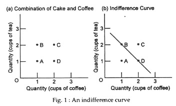
An indifference curve depicts the points of equally desirable combinations. Four combinations of tea and coffee are listed in the table. These are plotted in Figure 1 (a). Rationally preferring more to less, the consumer will surely prefer C to all other combinations. Combination C is preferred to B because C offers one more cup of coffee and the same amount of tea as B.
Combination C is preferred to A because C offers 1 more cup of tea and one more cup of coffee than A. And combination C is preferred to D because one more cup of tea is obtained with no loss of coffee. Combinations B and D are preferred to A; however, it is not possible to state whether B is preferred to D or D is preferred to B.
Let’s assume that the consumer has no preference between B and D. We thus say that the consumer is indifferent between combinations D (1 cup of tea and 2 cups of coffee) and combination B (2 cups of tea and 1 cup of coffee). Figure 1(b) shows that all combinations of goods among which the consumer is indifferent lie along an indifference curve.
By connecting points B and D, as in Figure 1(b), we trace out an indifference curve. An indifference curve shows all the combinations of two goods that will give the consumer the same level of total utility. If the consumer gets the same level of utility or satisfaction he will be indifferent (i.e., lacking any preference) among them.
The quantity of both the goods increases as the distance from the origin increases. Thus, any combination lying on the indifference curve (like B or D) is preferred to any combination falling below the curve, or closer to the origin (like A). Any combination appearing above the curve, or farther from the origin (like C), is preferred to any combinations lying on the curve.
Thus points A, B and C cannot lie on the same indifference curve; only points B and C can. Thus, indifference curves are always dense. In any particular commodity space (showing alternative combinations of any two goods) we can draw any number of indifference curves.
The Shape of Indifference Curves:
An indifference curve slopes downward from left to right, indicating that as less of one good is consumed, more of another good is consumed. It is based on the law of substitution, i.e., the consumption of one commodity is always at the expense of the other.
Indifference curves are not likely to be vertical, horizontal or upward sloping. They do not touch the axes and they do not touch each other.
ADVERTISEMENTS:
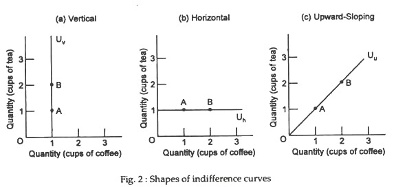
An indifference curve that is a vertical line, like the one labeled Uv in Fig. 2(a) would mean that the consumer is indifferent to combinations B and A. This is unlikely to happen in case of most goods, because combination B provides more of one good with no less of the other goods.
A vertical indifference curve, as in Fig. 2(a), would violate the condition that more is preferred to less as would a horizontal indifference curve, as shown in Fig. 2(b), or an upward sloping curve, like the one shown in Fig. 2(c). Thus, indifference curves are unlikely to have any of these shapes.
Similarly, horizontal indifference curves, such as line Uh in Fig. 2(b) are ruled out for most goods. People are not likely to be indifferent between combinations A and B along the horizontal curve since B provides more of one good with no less of the other good than A.
ADVERTISEMENTS:
An upward sloping curve, such as Uu in Figure 2(c) would mean that the consumer is indifferent between a combination of goods that provides less of everything and combination that provides more of everything (compare points A and B). A rational consumer will always prefer more to less.
The Slope of Indifference Curves:
Since the indifference curve approach is based on the law of substitution, the slope of an indifference curve is called the substitution ratio (or ratio of two marginal utilities): MUc/MUt. This is known as the marginal rate of commodity substitution.
An indifference curve slopes downward from left to right due to the law of substitution, i.e., due to the fact that the consumption of one commodity is always at the expense of the other if the consumer is to stay on the same indifference curve and enjoy the same level of utility or satisfaction.
ADVERTISEMENTS:
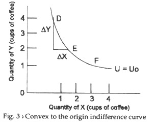
For a movement along the same indifference curve from point D to E we have,
Utility lost (by moving from D to D’) = Utility gained (by moving from D’ to E)
Or, – ∆Qc. MU = ∆Qt. MUC
Or, (∆C/∆T) = MUC/MUT
Convex to the Origin:
Indifference curves are convex to the origin. This means that as the consumer moves downward and to the right along the curve — a movement that implies increasing the quantity of coffee and reducing the quantity of tea — the curve becomes almost horizontal. This property is based on the law of substitution which seems to hold true in real life most of the time. The law of substitution may be stated as follows: The scarcer a good, the greater its relative substitution value; its marginal utility rises relative to the marginal utility of the good that has become abundant.
ADVERTISEMENTS:
In fact, the slope or steepness of indifference curves is determined by consumer preferences. The amount of one good that a consumer must give up to get an additional unit of the other good and remain equally satisfied changes as the consumer gives up one good to get the other. The less a consumer has of a good, the more the consumer values an additional unit of that good.
This preference is shown by an indifference curve that is convex to the origin, like the curve shown in Fig. 3. A consumer who has 4 cups of tea and 1 cup of coffee (point D) may be willing to give up 2 cups of tea for 1 more cup of coffee, moving from D to E.
But, a consumer who has only 2 cups of tea may be willing to give up only 1 cup to get that additional cup of coffee. This preference is shown as the move from E to F. In short, an indifference curve is convex in accordance with the empirical law of diminishing relative marginal utilities.
Indifference Curves Cannot Cross:
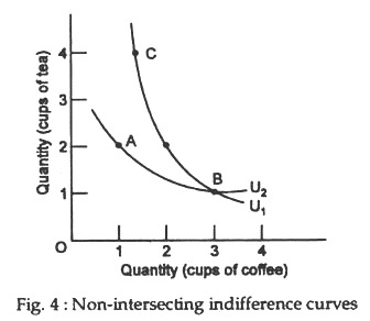
Indifference curves do not meet or intersect. If the curves crossed, two combinations of goods that are clearly not equally preferred by the consumer would seem to be equally preferred. As Fig. 4 shows the consumer is indifferent between A and B along indifference curve h and indifferent between B and C along indifference curve I1. Thus, the consumer appears to be indifferent among A, B and C. Combination C, however, offers more tea and no less coffee than combination A. Clearly the consumer, preferring more to less, will prefer C to A. Thus, indifference curves cannot cross.
An Indifference Map:
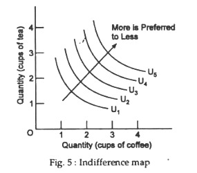
All the indifference curves in the commodity space together constitute the indifference map of the consumer. It is a complete set of indifference curves. An indifference map located in the positive quadrant of a graph indicates the consumer’s preferences among all combinations of goods and services. The farther from the origin an indifference curve is, the more the combinations of goods along that curve are preferred.
The arrow in Fig. 5 indicates the ordering of preferences. U2 is preferred to U1; U3 is preferred to U2 and U1, U4 is preferred to U3, U2 and U1, and so on. So, another important property of an indifference curve is that, an indifference curve which lies above and to the right of another indifference curve shows a preferred combination of the two commodities. This means that, any point in a higher indifference curve is always better than any point on a lower indifference curve.
Budget Line or Budget Constraint:
ADVERTISEMENTS:
The indifference map reveals only the combinations of goods and services that a consumer prefers or is indifferent among what he is willing to buy. It does not tell us what the consumer is able to buy. We may now ignore momentarily our representative consumer’s indifference map and give him (her) a fixed income. The consumers’ income level or budgets limit the amount that they can purchase.
Let us suppose he has Rs 6 per day to spend and he is faced with fixed prices for each unit of tea and coffee. It is quite obvious that he could spend his money on any of a variety of alternative combinations of tea and coffee. Fig. 6 shows the budget line or consumption possibility line. It is a locus of points showing all the combinations of goods that can be purchased with a fixed level of money income and at given prices.
Anywhere along the budget line in Fig. 6(a), the consumer is spending Rs 6. When the price of tea is Re 1 per cup and the price of coffee also Re 1 per cup, the consumer can choose among several different combinations of tea and coffee that add up to Rs 6. If only coffee is purchased, six cups of coffee can be purchased (point G). At point B, five cups of tea and one cup of coffee can be purchased. At point C, four cups of tea and two cups of coffee can be purchased. At point F, one cup of tea and five cups of coffee can be purchased.
The slope of the budget line is the ratio of the two prices. If daily expenditure is Rs 6, the following equation must hold: M = pxX + pyY or Rs 6 = Re 1 x Qc + Re 1 x Qt, where Qc and Qt denote quantities of coffee and tea bought. This is a linear equation, the equation of the budget line AG. Note that the arithmetic slope of AG = price of coffee + price of tea.
The equation of the budget line is:
ADVERTISEMENTS:
M = Pt. Qt + Pc. Qc
If the consumer buy only tea, the equation becomes M = Pt. Qt + 0 and the maximum amount of tea that he can buy is: Qt = M/Pt. Similarly, if the consumer buys only coffee the budget equation becomes M = 0 + Pc.
Qc, and there Qc = M/Pc.
So, the slope of the budget line is:
M/Pt ÷ M/Pc = M/Pt. Pc/M = Pt/Pc
An increase in the consumer’s income or budget is shown as a rightward shift of the budget line. Figure 6(b) shows an increase in income from Rs 6 to Rs 7. The budget line shifts out to the line running from 7 to 7. A change in income or in budget causes a parallel shift of the budget line.
A change in the price of one of the goods causes the budget line to change its slope. For example, with a budget of Rs 6 and the coffee at Re 1, we have the budget line Y1 of Figure 6(c). If the price of tea rises to Rs 2, only 3 cups of tea can be purchased if the entire budget is spent on tea. As a result, the budget line (Y2) becomes flatter, running from 3 on the vertical axis to 6 on the horizontal axis. Conversely, a rise in the price of coffee would cause the budget line to become steeper.
Consumer’s Equilibrium:
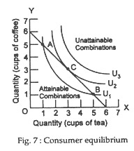
The indifference map shows the consumer’s desire to buy any two goods. The budget line shows his capacity to do so. He reaches equilibrium when his desire coincides with his capacity. So, by putting the budget line and the indifference map in the same diagram we can determine that particular combination of goods and services that the consumer is both willing and able to purchase. Any combination of goods that lies on or below the budget line is within the consumer’s budget. Which combination will the consumer choose in order to derive maximum satisfaction (utility)?
A rational consumer whose objective is utility maximisation will always try to reach the highest attainable indifference curve permitted by the budget line. The budget line in Fig. 7 indicates that most of the combinations along indifference curve U1 and point C on indifference curve U2 are attainable. Combinations along indifference curve U3 are preferred to combinations along U2, but the consumer is not able to buy combinations along because they cost more than the consumer’s budget.
Therefore, point C represents the maximum level of satisfaction or utility available to the consumer. Point C is the point where the budget line is tangent to (just touches) the indifference curve. Thus, consumer equilibrium is attained at the point where the budget line touches the highest attainable indifference curve. At that point the consumer’s satisfaction ratio (or the ratio of marginal utilities) is just equal to the ratio of the prices of the two goods.
This point may now be explained further. The substitution ratio, or the slope of the indifference curve, is the ratio of the marginal utility of coffee to the marginal utility of tea. So, at the tangency (equilibrium) point, the price of good and its marginal utility must be proportional. This means that in equilibrium the consumer is getting the same marginal utility from the last rupee spent on coffee as from the last rupee spent on tea.
We may, therefore, derive the following equilibrium condition:
Price ratio = Pc/Pt = Substitution ratio = MUc/MUt
Properties of Indifference Curves:
Indifference curves have four important properties:
1. An indifference curve which lies above and to the right of another shows a preferred combination of two goods.
2. An indifference curve slopes downward from left to right.
3. Two indifference curves cannot meet or intersect.
4. An indifference curve is convex to the origin.
Two of these are most important, because they relate to the shape of indifference curves. An difference curve is negatively sloped (downward sloping from left to right) and is convex to the origin (i.e., the marginal rate of substitution gradually diminishes as the consumer moves along the same indifference curve from left to right). Now, the shape we have assumed for the indifference curve plays a very important role in ensuring consumer equilibrium.
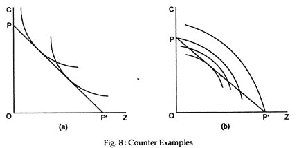
If any of the four properties of indifference curves were violated, consumer equilibrium would not be a tangency solution. Thus, if the first property were violated so that the consumer wished, say, to be on the lowest attainable indifference curve he would reach equilibrium at point P in Fig. 8(b), i.e., he would end up spending all his money on one commodity. If the second property were violated so that the slope of the indifference curves were not negative, there could be no point of tangency with the negatively sloping price line.
If the third property (non-intersect-ability of indifference curves) were violated, a number of points of tangency might occur [Fig. 8(a)] and if the indifference curves were concave to the origin, in violation of the fourth and last property, the point of tangency would yield the lowest attainable indifference curve, whereas the highest indifference curve would lie at one of the end points of the price line [P’ in Fig. 8(b)], so the rational consumer is at the point of minimum utility on his budget (price) line.
