Top 7 Applications of Indifference Curve Analysis

The following points highlight the top seven applications of indifference curve analysis. The applications are: 1. The Problem of Exchange 2. Effects of Subsidy on Consumers 3. The Problem of Rationing 4. Index Numbers: Measuring Cost of Living 5. Income-Leisure Trade-Off and Supply of Labour 6. The Effect of Income Tax vs. Excise Duty 7. The Saving Plan of an Individual.

Indifference Curve Analysis: Application # 1.

The Problem of Exchange:

With the help of indifference curve technique the problem of exchange between two individuals can be discussed. We take two consumers A and В who possess two goods X and Y in fixed quantities respectively. The problem is how they can exchange the goods possessed by each other.

This can be solved by constructing an Edge worth- Bowley box diagram on the basis of their preference maps and the given supplies of goods.

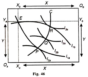
In the box diagram, Figure 46, O_a is the origin for consumer A and O_b the origin for consumer В (turn the diagram upside down for understanding). The vertical sides of the two axes, O_a and O_b, represent good Y and the horizontal sides, good X.

The preference map of A is represented by the indifference curves I₁a, I₂a, 13a and B’s map by I₁b, I₂b and 1₃b indifference curves. Suppose that in the beginning A possesses O_a Y_a units of good Y and O_a X units of good X. В is thus left with O_AY_A of Y and O_b X_b of X. This position is represented by point E where the curve I₁a intersects I₁b.

Suppose A would like to have more of X and В more of T. Both will be better off, if they exchange each other’s unwanted quantity of the good, i.e. if each is in a position to move to a higher indifference curve. But at what level will exchange take place? Both will exchange each other’s good at a point where the marginal rate of substitution between the two goods equals their price ratios.

This condition of exchange will be satisfied at a point where the indifference curves of both the exchangers touch each other. In the above figure P, О and R are the three conceivable points of exchange. A line CC passing through these points is the “contract curve” or the “conflict curve”, which shows the various positions of exchange of X and Y that equalize the marginal rates of substitution of the two exchangers.

If exchange were to take place at point P then consumer В would be in an advantageous position because he is on the highest indifference curve l₃b. Individual A would, however, be at a disadvantage for he is on the lowest indifference curve l₁a. On the other side, at point R, consumer A would be the maximum gainer and В the loser.

However, both will be at an equal position of advantage at Q. They can reach this level only by mutual agreement; otherwise the point of exchange depends upon the bargaining power of each party. If A has better bargaining skill than B, he can push the latter to point R. Contrariwise, if В is more skilful in bargaining he can push A to point P.

Indifference Curve Analysis: Application # 2.

Effects of Subsidy on Consumers:

The indifference curve technique can be used to measure the effects of government subsidy on low income groups. We take a situation when the subsidy is not paid in money but the consumers are supplied cereals at concessional rates, the price-difference being paid by the government.

This is actually being done by the various state governments in India. In Figure 47 income is measured on the vertical axis and cereals on the horizontal axis.

Suppose the consumer’s income is OM and his price-income line without subsidy is MN. When he is given subsidy by supplying cereals at a lower price, his price-income line is MP (it is equivalent to a fall in the price of cereals). At this price-income line, he is in equilibrium at point E on curve I₁ where he buys OB of cereals by spending MS amount of money.

The full market price of OB cereals is MD on the line MN where the curve I₀ touches. The government, therefore, pays SD amount of subsidy. But the consumer receives cereals at a lower price. He does not receive SD amount of subsidy in cash. If the money value of the subsidy were to be paid to him in cash, they would receive MR amount of money.

The equivalent variation MR shows that in the absence of the subsidy, a cash payment would bring the consumer on the same indifference curve, which makes him as better off as the subsidy. But the value of the subsidy MR to the consumer is smaller than the cost of the subsidy DS to the government. It reveals the fact that the consumer is happier if he is paid the subsidy in cash rather than in the form of subsidized cereals.

In this case, the cost of subsidy to the exchequer will also be less. It points out to another interesting result. When the income of the consumer is raised by giving him cash subsidy, he will buy less cereal than before. In Figure 47 at the equilibrium point C, he buys OA of cereals which are less than OB when he was getting them at the subsidized price. This is what the government actually wants.

Indifference Curve Analysis: Application # 3.

The Problem of Rationing:

The indifference curve technique is used to explain the problem arising from various systems of rationing. Usually rationing consists of giving specific and equal quantities of goods to each individual (we ignore families because equal quantities are not possible in their case).

The other, rather liberal, scheme is to allow an individual more or less quantities of the rationed goods according to his taste. It can be shown with the help of indifference curve analysis that the latter scheme is definitely better and beneficial than the former.

Let us suppose that there are two goods rice and wheat that are rationed, the prices of the two goods are equal and that each consumer has the same money income. Thus, given the income and price-ratios of the two goods, MN is the price-income line. Rice is taken on vertical axis and wheat on the horizontal axis in Figure 48.

According to the first system of rationing, both consumers A and В are given equal specific quantities of rice and wheat, OR + OW. Consumer A is on indifference curve l_a and В is on I_y with the introduction of the liberal scheme each can have more or less of rice or wheat according to his taste.

In this situation, A will move from P to Q on a higher indifference curve I_b1. Now he can have OR_A of rice +OW_a of wheat. Similarly, В will move from P to R on a higher indifference curve I and can buy OR_b of rice +OW_b of wheat.

With the introduction of the liberal scheme of rationing both the consumers derive greater satisfaction. The total quantity of goods sold is the same. For when В buys more quantity of wheat WW_b , he purchases less quantity of rice RR_b and when A buys RR_a more of rice, he purchases WW less of wheat.

Thus, the governmental aim of controlled distribution of goods is not disturbed at all; rather there has been a better distribution of goods in accordance with individual tastes.

Indifference Curve Analysis: Application # 4.

Index Numbers: Measuring Cost of Living:

The indifferent curve analysis is used in measuring the cost of living or standard of living in terms of index numbers. We come to know with the help of index numbers whether the consumer is better off or worse off by comparing two time periods when the income of the consumer and prices of two goods change.

Suppose a consumer buys only two goods X and Y in two different time periods 0 and 1 and he spends his entire income on them in the two periods. It is also assumed that the consumer’s tastes and quality of the two goods do not change.

There are two standard methods of measuring changes in the price level: the Laspeyres and the Paasche index

This is represented by the new budget line CD. This line passes through point L which shows that the initial combination ОХ₀-ОУ₀ of the two goods is available to the consumer at the new price – income ratio on the I₀ curve. But he can be on the higher indifference curve I₁ at point L₁ on the budget line CD and have the combination OX and OY₁ of the two goods.

Since both L and L₁ lie on the new budget line CD, both the combinations have the same cost. But the consumer will choose the combination L₁ because it is on the higher indifference curve I₁ and he is better off in period 1 than in the base period 0.

Now take the Paasche price index where the initial budget line in Figure 50 is AB in the base period 0 and the consumer is in equilibrium at point P on the indifference curve I₀ .The new budget line in period 1 is CD which passes through point P₁ on the new indifference curve I₁.

Both the combinations P and P₁ lie on the original budget line AB. Therefore, they have the same cost. But combination P is on the higher indifference curve I₀ than combination P₁ However, the consumer cannot have combination P₁ on the lower indifference curve I₁, and is worse off in period I than in the base period 0.

Indifference Curve Analysis: Application # 5.

Income-Leisure Trade-Off and Supply of Labour:

The indifference curve technique is used to explain some of the problems of the individual supply of labour such as the income-leisure trade-off, high overtime rates and the backward-sloping supply curve of labour.

Income-Leisure Trade-Off:

A worker’s offer to supply his labour depends on his preferences between income and leisure and the wage rate. Income and leisure are inversely related, whereas there is a direct relationship between incomes and hours worked per day. Leisure is always exchanged for income.

This analysis assumes that there are no institutional constraints on working hours and the workers are free to work or have leisure. Decisions about working hours are analysed by constructing an indifference map relating income to leisure. An indifference curve shows different combinations of income and leisure that would be acceptable to a worker.

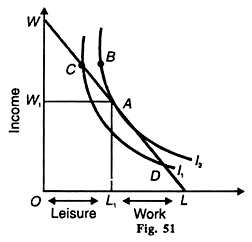
Figure 51 measures income (or wages) on the vertical axis and leisure and work time on the horizontal axis. The income-leisure indifference curve is I₂. The line WL is the income-leisure line of the worker. The wage rate (w) is equal to the slope of this line.

The line WL indicates that if he does not work at all, he enjoys OL hours of leisure and earns zero income, and if he works for OL hours, he earns the maximum income OW. But what point he will actually choose on his income – leisure constraint line WL? To answer this question, let us consider a worker who has Я hours available to him daily and he devotes L hours out of them to work.

If we denote his leisure or free hours by F, then

L = H—F which is the number of hours he works.

If the wage rate is w, then his income у is y=wL

and his income-leisure choice can be given by

y = wH – wF

If the worker’s objective in making his income-leisure choice is to maximise his satisfaction, he will choose that combination of income-leisure where his income-leisure line is tangent to his indifference curve. In Figure 51, it is point A at which the curve 1₂ touches the WL line. Given the wage rate, the worker gets maximum Fig. 52 satisfaction by working L₁L hours, earning OW₁ income and enjoying ОL₁ hours of leisure.

If the worker tries to move away from point A to point В on the I₂ curve, it would yield the same level of satisfaction. But point В is unattainable because it lies above his income-leisure line WL. In fact, all points on I₂ other than A are unattainable, But these points lie on the lower indifference curve I₁ indicating a lower level of satisfaction.

Therefore, any move away from point A will not give him maximum satisfaction. Hence he will choose only combination A of income-leisure.

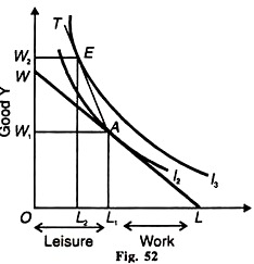
Now consider a case when a worker is offered an overtime wage rate so that he works some additional hours. This is illustrated in Figure 52 by drawing a steeper income-leisure line to the left of point A so that this line has kink at this point.

Such a line is AT whose slope shows that the overtime wage rate is higher than the wage rate shown by the slope of the line WL. The worker is in equilibrium at point E where the higher indifference curve I₃ is tangent to the line AT. Now the worker works L₂ L hours by earning OW₂ income as against L₁L hours of work and OW₁ of income earlier. Thus the worker has earned W₁W₂ additional wage by working L₂L₁ overtime hours.

 

The Supply of Labour:

The supply curve of an individual worker can also be derived with the indifference curve technique. His offer to supply labour depends on his preference between income and leisure and on the wage rate. In Figure 54 hours of work and leisure are measured on the horizontal axis and income or money wage on the vertical axis. W₁L is the wage line or income-leisure line whose slope indicates wage rate (w) per hour.

When the wage rate increases, the new wage line becomes W₂ L and the wage rate per hour also increases and similarly for the wage line W₃L. As the wage rate per hour increases, the wage line becomes steeper. When the worker is in equilibrium at the tangency point E₁ of wage line W₁L and indifference curve I₁, he earns E₁L₁ wage by working L₁L hours and enjoys OL₁ of leisure.

Similarly, when his wage increases, to E₂ L₂, he works for longer hours L₂ L and with E₃ L₃ wage increase, he works for still longer hours L₃ L and enjoys lesser and lesser leisure than before. The line connecting the points E₁E₂ and E₃ is called the wage-offer curve.

The supply curve of labour can be drawn from the locus of the equilibrium points E₁ E₂ and E₃ But the wage-offer curve is not the supply curve of labour . Rather, it indicates the supply curve of labour. To derive the supply curve of labour from the wage-offer curve given in Figure 54, we draw the wage-hour schedule in Table 8.

On the basis of the above schedule, the supply curve of labour is drawn in Figure 54 where the wage rate per hour is plotted on the vertical axis and hours worked (or supply of labour) on the horizontal axis. When the wage rate is W₁, labour supplied is OL₁ As the wage rate rises to W₂, and W₃ , labour supplied increases to OL₂ and OL₃ respectively.

The wage-labour combination points E₁ E₂ and Е, trace out the supply of labour curve SS₁ The SS₁ curve is positively sloping upwards from left to right which shows that when the wage rate increases, the worker works for more hours.

This attitude of the worker is the result of two forces: one, the substitution effect, and two, the income effect of the wage increase. When the wage rate increases, the tendency to work longer hours increases on the part of the worker in order to earn more. It is as if leisure has become more expensive. So the worker has a tendency to substitute work for leisure. This is the substitution effect of the wage increase.

Further, when the wage rate increases, the worker becomes potentially better off, he has a feeling of satisfaction and gives preference to leisure over work. This is the income effect of the wage increase. In the figure, as the wage rate increases from to W₂ and to W₃, hours worked increase from OL₁ to OL₂ and to OL₃ This is because the substitution effect of wage increase is stronger than the income effect.

Backward-Sloping Supply Curve of Labour:

At some higher wage rate if the wage rate increases further, the worker may work for lesser hours and enjoy more leisure. This case is illustrated in Figure 55. When the income of the worker increases progressively from E₁L₁ to E₁ L₂ and to E₃ L₃, hours worked may decline at some level of income.

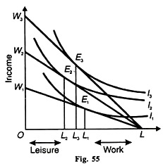
At the equilibrium point E₁ hours worked are Lf and they increase to L₂L at the equilibrium point E₂ when his income rises to E₂L₂ from E₁L₁ .But further increase in income to E₃ L₃ leads to the reduction in hours worked to L₃L from L₂L.

The worker now increases his leisure hours from OL₂ to OL₁ .The corresponding supply curve of labour is drawn in Figure 56 which is backward slopping. Taking the substitution effect and the income effect of the wage increase up to the wage rate W₂, the substitution effect is stronger than the income effect.

So the supply curve of this worker is positively sloped from S to E₂ At the wage rate W₂ , the substitution effect exactly equals the income effect and the SS, curve is vertical at point E₂.

As the wage rate increases above W₂, the income effect is stronger than substitution effect and the supply curve is negatively sloped in the region E₂S₁ which shows that the worker gives preference to leisure over work. In the figure, when the wage rate increases to W₃ the worker reduces his hours worked from OL₂ to OL₃ and thus enjoys L₂L₃ of leisure.

Indifference Curve Analysis: Application # 6.

The Effect of Income Tax vs. Excise Duty:

The indifference curve technique helps in considering the welfare implications of income tax vs. excise duty or sales tax. Whether an income tax hurts the tax payer more or an excise duty of an equal amount? Let us take a taxpayer who is required to pay, say Rs 4000 annually either as income tax or as excise tax on a commodity X.

It is further assumed that he will continue to buy the commodity even after the imposition of the duty when its price goes up.

In Figure 57 the money income of the taxpayer is shown along the vertical axis. He has OM of income and his original price-income line, before the tax is levied, is MN. He is in equilibrium at point В on the indifference curve I₁. For MA quantity of X, he spends AB.

Now when the excise duty on commodity X is levied, its price rises so that his price-income line shifts to MN\ where he is in equilibrium at point С on the I₂ curve. As a result of the tax, he buys ML quantity of X and spends LC on it. But at the original price, this quantity ML would have cost him LS. Thus SC is the amount of tax which he pays for it.

If an equal amount of tax is raised by the government through income tax instead, the taxpayer’s income would be reduced by MT (=SC). He moves to a lower line TR on the indifference curve I₃ at point D. Since the indifference curve I₃ is higher than I₂, the income tax equivalent to an excise duty places the taxpayer in a favourable position.

Indifference Curve Analysis: Application # 7.

The Saving Plan of an Individual:

The indifference curve technique can also be used to study the saving plan of an individual. An individual’s decision to save depends upon his present and future income, his tastes and preferences for present and future commodities, their expected prices, on the current and future rate of interest, and on the stock of his savings.

As a matter of fact, his decision to save is influenced by the intensity of his desire for present goods and future goods. If he wants to save more, he spends less on present goods, other things being equal. Thus saving is, in fact, a choice between present goods and future goods. This is illustrated in Figure 58 with the help of indifference curves.

Let PF₁ be the original price-income line of the individual where he is in equilibrium at point S on the indifference curve I. Given the price of the present and future goods, the income of the consumer, his tastes and preferences for the present and the future, and the rate of interest, he buys OA of the present goods and plans to save so much as to have OB of goods in the future.

Suppose there is a change in his preferences. What will be the effect of such a change on the consumer’s saving plan? If his preference for the present goods increases, his price-income line will move to P₁F so that he is in equilibrium at point Q on I₁ He now buys OA₁ present goods and thus saves less for the future goods.

As a result, the purchase of the future goods will fall from OB to OB₁. On the other hand, if in his estimation the value of future consumption increases, his price-income line will move to P₂F₂ where he will be in equilibrium at point R on I₂ curve.

He will, therefore, save more and thus reduce his consumption of present goods to OA₂ in order to have OB₂ future goods. Similar effects can be traced if the rate of interest changes, other things remaining constant.