
Indifference Curve Applications of Taxes and Subsidies!
Indifference Curve Applications:
Income Tax vs. Excise Tax:
Indifference curve analysis may be applied to compare the effects of two different taxes, viz., an income tax and an excise tax. We shall see that the typical consumer is better off with an income tax than with a comparable excise tax on a single commodity.
Let us suppose that the consumer buys only two goods, X and Y. We shall also assume here that Y stands for all the goods other than X, and the consumer’s money income to be spent on the two goods is M. We shall discuss the effects of the taxes with the help of Fig. 6.94, where AB is the pre-tax budget line of the consumer. Let us now suppose that an excise tax is imposed on good X.

If the sellers can pass on the whole tax to the consumers, the price of X will rise by the amount of the tax, and the x-intercept of the budget line will reduce from OB to OB1, and the post-tax budget line would become AB1.
ADVERTISEMENTS:
The consumer’s equilibrium before the imposition of the tax was at the point of tangency C between the budget line AB and one of his indifference curves (ICs), IC3, and now it would be at the point of D where the post-tax budget line AB1 has touched IC1 which is a lower curve than IC3.
Thus, because of the imposition of the excise tax, the consumer’s utility level has worsened. This is what is expected, because the imposition of the tax has caused an increase in the price of one of the two goods, viz., X, that the consumer buys.
We may now obtain the revenue obtained from the tax, which is equal to the reduction in the amount of money spent on the two goods by the consumer, due to the imposition of the tax.
ADVERTISEMENTS:
The consumer’s income at any point H on his pre-tax budget line is equal to the money he spends on x and Y which is, therefore, equal to FH.px + OF.py. On the other hand, the total amount of money he spends on the two goods at the point D is FD.px + OF.pY. Therefore, the amount he pays in tax is equal to (FH.px + OF.py) – (FD.px + OF.pY) = (FH – FD)px = DH.px.
Let us now come to the effects of an income tax upon the economic well-being of the consumer. In order to make the effects of an income tax comparable with those of an excise tax, we shall assume that the consumer would be asked to pay an income tax of the same amount as the excise tax which, in our case, is DH.px in Fig. 6.94.
Now, if the consumer is asked to pay an income tax of the amount DH.px in terms of money, or, DH.px/px = DH in terms of good X, then, prices of the goods remaining the same, his pre-tax budget line AB would have a horizontal and parallel leftward shift by an amount of DH = B2B.
That is why the post-income tax budget line of the consumer would be A2B2— it would pass through the point D. Now, the consumer would be in equilibrium at the point of tangency E between the budget line A2B2 and the curve IC2.
ADVERTISEMENTS:
Since, IC2 is a lower curve than IC3, consumer’s level of satisfaction will be adversely affected by the income tax, but since IC2 is a higher curve than IC1 his well-being will not be as adversely affected as done by the excise tax. We may conclude, therefore, that the consumer is better off with an income tax than with a selective excise tax on good X.
Let us note that his consumption of X is higher under the income tax than under the excise tax (GE > FD), since, under the excise tax, he is at the point D, but under the income tax, he has further opportunity to maximise in the region of the triangle DB1B2.
Income Subsidy vs Price Subsidy:
Indifference curves may be used to analyse the effects of an income subsidy and a price subsidy upon the utility level of the consumer. An example of a price subsidy is obtained when the government pays, say, 80 per cent of the cost of medical care which means actually an 80 per cent reduction in the price of medical care.
Another example is the Food Stamp Programme in the USA before 1979. Low-income families had to pay, say, $ 20 to buy $ 60 worth of food stamps. This is equivalent to two-thirds reduction in the price of food. A comparison between an income subsidy and a cash subsidy may be illustrated with the help of Fig. 6.95.

Here we have assumed that the consumer purchases only two goods, X and Y, and his money income is M. Initially, let us suppose that the budget line of the consumer is AB and his equilibrium is at the point of tangency C on the indifference curve, IC1.
Let us now suppose that the consumer is given an income subsidy of amount, say, S. This implies that now his income would increase, from M to M + S. As the consumer now spends more money, prices of the goods remaining unchanged, his budget line would have a parallel horizontal shift to the right from AB to A1B1, and his income would increase by BB1 in terms of x, or, S in terms of money, and his equilibrium point would move from Point D is the point of tangency between the budget line A1B1 and the curve IC3.
Since IC3 is a higher curve than IC1 the income subsidy improves the utility level of the consumer. Let us now consider the effects of a price subsidy on good X upon the well-being of the consumer.
With a view to making the effects of a price subsidy comparable with those of an income subsidy, we shall assume that the consumer would be given a price subsidy that would enhance his total expenditure in terms of x by an amount which is the same as that of the income subsidy.
ADVERTISEMENTS:
In our case, this amount is BB1 along the horizontal axis. After the consumer receives the price subsidy on X, his expenditures in terms of x would be OB1 and those in terms of y would be OA, prices of the goods remaining the same.
Therefore, now the consumer’s budget line would be AB1 and he would be in equilibrium at the point of tangency E between this budget line and an IC, viz., IC2. Since IC2 is a higher curve than IC1, the price subsidy increases his well-being but since IC2 is lower than IC3, his well-being will not improve as much as in the case of cash subsidy.
We may conclude, therefore, that the consumer is better off with a cash subsidy than with a selective price subsidy on a single good.
Cash Subsidy vs Subsidy in Kind: The Food Stamp Programme:
In the case of a cash subsidy the consumer is given some amount of cash as a matter of subsidy. He can use the cash in buying the goods according to his will. On the other hand, if an equal amount of subsidy is tied to a good, say X, then it is known as a subsidy in kind or an in-kind subsidy.
ADVERTISEMENTS:
In the case of subsidy in kind, the consumer receives as subsidy an amount of the good (X) that can be bought with the subsidy. Food stamp Programme in the USA (after 1979) is an example of in-kind subsidy. Under this programme, the low-income families receive food stamps which they can use to purchase food only.
The stamps are non-tradable (if they were tradable, then the programme would have reduced to a general cash subsidy programme). We may compare the effects of cash subsidy and in-kind subsidy upon the consumer’s utility level with the help of Fig. 6.96. We shall assume here that the prices of goods X and Y remain unchanged as also the consumer’s initial money income, throughout our analysis.
In Fig. 6.96(a) AB is the budget line of the consumer before he receives any form of subsidy. When the consumer receives a cash subsidy this would boost up his income, the prices of the goods remaining unchanged. Consequently, his budget line would have a parallel rightward shift from AB to, say, A1B1. The amount of cash subsidy here is BB1.px, or, AA1.py.
However, if the consumer receives an equal amount of in-kind subsidy, i.e., BB1 of good X, the x-intercept of his initial budget line AB would become OB1 (= OB + BB1), i.e., if buys nothing of good Y, he would have OB, of good X. On the other hand, if he spends all his money income on Y, he would have OA of Y plus he would be able to buy an amount of X with the subsidy which is equal to BB1 or AC.
ADVERTISEMENTS:
Therefore, now, the consumer’s budget line would become AC B1 in Fig. 6.96(b). Of course, his effective budget line now would be the line segment CB1 for he would never remain at any point on the segment AC, because that would mean he is not drawing the full advantage of the subsidy which a utility-maximising rational consumer cannot do.
Now that we have obtained the budget lines of the consumer in the cash subsidy and in-kind subsidy cases, it would be rather easy for us to compare between the effects of the two cases upon the consumer’s utility level.
We shall see in Fig. 6.96 that the effects of the two types of subsidy would depend upon the preference-indifference pattern of the consumer, i.e., upon the position of his indifference curves (ICs). In each of parts (b), (c) and (d) of Fig. 6.96, the pre- subsidy equilibrium of the consumer has occurred at the point E where the consumer’s budget line AB has touched one of his ICs, viz., IC1.

Now in the post-subsidy situation in Fig. 6.96(b), both the cash and in-kind subsidy budget lines A1C B1 and ACB1, have touched the same IC, viz., IC2, at the point F. Therefore, both types of subsidy will take the consumer from the point E on IC1 to the point F on IC2, which is a higher curve.
Therefore, in this case, both the subsidies will improve the consumer’s utility level in the same way, i.e., the effects of both types of subsidy will be identical. Therefore, the consumer will be indifferent between the two types of subsidy.
ADVERTISEMENTS:
In Fig. 6.96(c), the positions of the ICs are slightly different. But this difference is irrelevant, for we get the same effects as in the previous case. Here an IC, viz., IC2, has touched the budget line ACB1 at the point C and, at the same time, it has touched the budget line ACB1 at its corner point C.
Therefore, in both cases, the consumer’s equilibrium point will move from the point E on IC1 to C on IC2, which is a higher curve. Therefore, in both types of subsidy, the effect would be the same type of improvement in the utility level of the consumer, and he would be indifferent between them.
Lastly, in Fig. 6.96(d), the position of the ICs makes the post-subsidy situations qualitatively different from the previous two cases. Here the consumer equilibrium occurs at the corner point, C1 of the in-kind subsidy budget line ACB1 on IC2.
However, in the case of the cash subsidy budget line ACB1 equilibrium occurs on a higher IC, viz., IC3 at the point H. Therefore, in this case, the consumer would prefer the cash subsidy to the in- kind subsidy. We have compared the effects of a cash subsidy and an in-kind subsidy upon the economic well-being of the consumer.
We have examined three different situations in Fig. 6.96—(b), (c) and (d) the consumer will never be worse off and sometimes he will be better off, as in the case of Fig. 6.96 (d), with a cash subsidy.
This is because the segment A1C of the cash subsidy budget line or the consumption possibility line A1CB1 is not available to the consumer when he receives the in-kind subsidy, but the whole of the effective segment CB1 of the in-kind subsidy budget line is also open to the consumer when he receives the cash subsidy.
ADVERTISEMENTS:
Therefore, every individual consumer who takes the prices as given will prefer a cash subsidy to an in-kind subsidy, unless there is any other consideration.
Taxes on Cash Subsidy:
We have concluded that an individual consumer will always prefer cash subsidy to an in-kind subsidy. However, if there is any other consideration, e.g., if a tax is imposed on the cash subsidy, but not on the in-kind subsidy, then we may be required to change this conclusion. We may explain the matter with the help of Fig. 6.97.
The post-subsidy budget lines without any sort of tax are A1CB1 for cash subsidy and ACB1 for in-kind subsidy in Fig. 6.97(a), just as they were in Fig. 6.96(a). Let us now suppose that a tax is imposed on cash subsidy, but not on the in-kind subsidy. Consequently, the cash subsidy budget line, net of tax, will be A2B2—it would be to the left of A1B1 but parallel to it because the prices remain unchanged.
The in-kind subsidy budget line, however, would remain the same as ACB1. In Fig. 6.97(a), the ICs of the consumer are positioned in such a way that, with the in-kind subsidy without any tax the consumer is in equilibrium at the point of tangency F on a higher IC, viz., IC2 and with cash subsidy, net of tax, the consumer is in equilibrium at the point of tangency E on a lower IC, viz., IC1. Therefore, the consumer here will prefer the in-kind subsidy to the (taxed) cash subsidy.
Fig. 6.97(b) illustrates the case where the ICs of the consumer are so positioned that he will prefer the cash subsidy even if taxed to the untaxed in-kind subsidy. Here, with cash subsidy net of tax, the consumer is in equilibrium at the point G which is the point of tangency between the cash subsidy, net of tax, budget line A2B2 and IC2.

On the other hand, with in-kind subsidy, untaxed, the consumer is in equilibrium at the corner point C which lies on IQ. Since IC2 is a higher curve than IC1, the consumer would even prefer a taxed cash subsidy to the untaxed in-kind subsidy.
ADVERTISEMENTS:
Indifference Curve Applications—Intertemporal Choice in Consumption:
Introduction:
The consumption function introduced by Keynes (1883-1946) relates current consumption to current income. This relationship, however, is incomplete at best. For when people decide how much to consume and how much to save, they consider both the present and the future.
The more consumption they enjoy today, the less they will be able to enjoy tomorrow. In making this trade off, households must look ahead to the income they expect to receive in the future and to the consumption of goods and services they hope to be able to afford.
Here we shall discuss the model developed by Irving Fisher (1867-1947) to analyse how rational, forward-looking consumers make inter-temporal choices, i.e., choices regarding consumption between different periods of time.
ADVERTISEMENTS:
Fisher’s model focuses on the constraints the consumers face, the (ordinal) preferences they have, and how these constraints and preferences together determine their choices about consumption and saving. The model may be considered to be an application of the indifference curve theory.
The Intertemporal Budget Constraint:
Most people would prefer to increase the quantity or quality of the goods and services they consume. But people consume less than they desire because their consumption is constrained by their income. In other words, the consumers face a constraint on how much they can spend, which is called a budget constraint.
But when they decide how much to consume today versus how much to save for the future, they face an inter-temporal budget constraint, which measures the total resources available for consumption today and in the future. We shall first examine this constraint in some detail.
To keep things simple, we shall examine the decision facing a consumer who lives for two periods. Period 1 represents the consumer’s youth and period 2 represents the consumer’s old age. The consumer earns income Y1 and consumes C2 in period 1, and earns income Y2 and consumes C2 in period 2.
(All variables are real, that is, adjusted for inflation) Because the consumer has the opportunity to borrow and save, consumption in any single period can be either greater or less than income in that period.
Let us consider how the consumer’s income in the two periods imposes constraints upon his consumption in these periods. In period 1, saving equals income minus consumption, i.e.,
S=Y1-C1 ………(6.131)
where S is saving.
In period 2, consumption equals the accumulated saving, including the interest earned on that saving, plus period 2 income.
That is:
C2 = (1 + r) S + Y2 ……….(6.132)
where r is the real rate of interest. It may be noted that the consumer here does not save in the second period because there is no third period.
Let us also note that the variable S can represent either saving or borrowing (negative saving) and equations (6.131) and (6.132) hold in both cases. If period-1 consumption is less than period-1 income, the consumer is saving (S > 0).
On the other hand, if period-1 consumption exceeds period-1 income, the consumer is borrowing (S < 0). For simplicity, we shall assume here that the interest rate for borrowing is the same as the interest rate for saving.
In order to derive the consumer’s budget constraint we have to combine equations (6.131) and (6.132) and thereby we obtain
![]()
Eqn. (6.134) gives us the standard form of the consumer’s inter-temporal budget constraint. This constraint can be easily interpreted. If the interest rate is zero (r = 0), total consumption in the two periods equals total income in the two periods: (Q + C2 = Y1 + Y2).
In the usual case, when r > 0, future consumption and future income are discounted by a factor 1 + r. This discounting arises from the interest earned on saving. If the consumer does not save in period 1, then also we have C1 = Y1 and C2 = Y2 giving us C1 + C2 = Y1 + Y2.
In essence, because the consumer earns interest on current income that is saved, future income is worth less than current income, i.e., the consumer would prefer to have more of current income to more of future income.
Similarly, because any particular quantity of future consumption is paid for out of savings that have earned interest, future consumption costs less than current consumption.
The factor 1/1+r which is equal to the reciprocal of the numerical slope of the budget line (6.134), is the price of period 2 consumption measured in terms of period 1 consumption—it is the amount of period 1 consumption that the consumer must forego to obtain one unit of period 2 consumption.
Fig. 6.98 graphs the consumer’s budget constraint. At point A on the budget line, the consumer consumes exactly his income in each period (C1 = Y1 and C2 = Y2), so there is neither nor borrowing between the two periods. At point B, the consumer consumes nothing in period 1 (Q = 0) and saves all income, so the period-2 consumption is C2 = (1 + r) Y1 + Y2.
At point D, the consumer plans to consume nothing in period 2 (C2 = 0) and he borrows in period-1 as much as possible against period-2 income. So period-1 consumption would be C1 = Y1 + Y2/1+r. Of course, A, B and D are only three of the many combinations of period-1 and period-2 consumption that the consumer can afford; consumption at any point on the line from B to D is available to the consumer.

Consumer Preferences:
The consumer’s preferences regarding consumption in the two periods can be represented by his indifference curves (ICs). An IC shows the combinations of period-1 and period-2 consumption that make the consumer equally happy so that he would be indifferent between these combinations.
Fig. 6.99 shows two of the consumer’s many ICs. The consumer is indifferent among combinations W, X and Y on IC1 because they are all on the same curve. An IC here is negatively sloped. This is not at all surprising, because both C1 and C2 are MIBs—if the consumer’s period 1 consumption is reduced to, say, from point W to point X, his period-2 consumption must increase to keep him equally happy.

The numerical slope at any point on an IC of Fig. 6.99 gives us how much period 2 consumption (i.e., C2) he may forego for a small one unit increase in period 1 consumption (i.e., C1). This numerical slope, as we know, is known as the marginal rate of substitution of C1 for C2. It tells us the rate at which period 1 consumption would be substituted for period-2 consumption at any particular point on the IC, or, at any particular C1.
The ICs of Fig. 6.99 are not straight lines. They are convex to the origin. This is because of our assumption that as the consumer goes on substituting C, for C2, i.e., as he slopes downward towards right along an IC, his MRS of C1 for C2 would decrease, i.e., as his period-1 consumption (C1) increases he would be willing to forego less and less of period-2 consumption. This is known as diminishing MRS of Q for C2.
Lastly, the consumer is equally happy at all points on an IC but he prefers any point on a higher IC to any point on a lower IC. This is because the consumer is assumed to prefer more of C1 and/or C2 to less of C1 and/or C2 and any point on a higher IC is a combination of more of one or both of C1 and C2 than some point or points on a lower IC.
Because of this last property of the ICs, the consumer would always prefer to reach the highest possible IC, or the highest possible level of satisfaction subject to his inter-temporal budget constraint.
Equilibrium of the Consumer:
Because of the shape of the consumer’s ICs and that of his budget constraint, he would achieve the highest possible level of satisfaction at c, the point of tangency between his budget line and one of his ICs. This point of tangency is the point Q on IC3 in Fig. 6.100.

Since, at the optimum point or the point of tangency, the numerical slope of the IC is equal to that of the budget line, and since, the former is equal to MRS of C) for C2 and the latter is equal to 1 + r, the consumer’s optimum or equilibrium point is characterised by:
MRC1 for C2 = 1 + r (6.35)
That is, the consumer chooses consumptions in period 1 and period 2, i.e., (C01, C02), so that the MRS equals 1 plus the real interest rate (r).
Effect of a Change in Income upon Consumption:
Let us now see how consumption responds to an increase in income. An increase in Y1 and/or Y2, r remaining unchanged, leads to a rise in both the intercepts of the budget line, viz., Y1 + (Y2/1+r) and (1 + r) Y1 + Y2, the slope of the budget line remaining the same.
As a result, there would be an outward parallel shift in the budget line. This new budget line would touch a higher IC. A ceteris paribus rise in (real) income would cause a rise in the consumer’s happiness which is reflected in the fact that the consumer’s optimum point now would be on a higher IC.
This is shown in Fig. 6.101. Here the initial optimum point of the consumer is Q1 and the new equilibrium point after a parallel outward shift of the budget line is Q2.
If we assume that both C1 and C2 are normal goods, then both would in- c, crease after an increase in income and the consumer’s new equilibrium point Q2 would be positioned upward towards right of his initial equilibrium point Q1. This has been the case in Fig. 6.101.

The important conclusion that we can make here is that regardless of whether the increase in income occurs in period 1 or in period 2, the consumer spreads it over consumption in both periods. This behaviour is called consumption smoothing.
Because the consumer can borrow and lend between periods, the timing of the income is irrelevant to how much is consumed today or tomorrow. The lesson of this analysis is that consumption depends on the present value of current and future income i.e., on present value of income which is
![]()
Let us notice that this conclusion is quite different from that reached by Keynes. Keynes assumed that a person’s current consumption depends largely on his current income. But Fisher’s model says, instead, that consumption is based on the resources the consumer expects to have over his lifetime.
Effect of a Change in the Real Interest Rate (r) upon Consumption:
We may now use Fisher’s model to consider how a change in the real interest rate (r) may alter the consumer’s choice. There are two cases to consider. First, the case in which the consumer is initially saving, and second, the case in which he is initially borrowing.

We shall first discuss the saving case with the help of Fig. 6.102. Here, the consumer’s initial budget line is L1M1 and A (Y1, Y2) is a point on it. This line has touched one of his ICs, viz., IC1 at the point D(C’1, C’2). D is, therefore, the consumer’s initial equilibrium point. Since the consumer is a saver in period 1, we have, C’1 < Y1 and C’2 > Y2, i.e., the point D would lie upward towards left of point A.
Let us now suppose that r rises, Y1 and Y2 remaining unchanged. Consequently, the horizontal (CO intercept of the budget line, i.e., Y1 + Y2/ (1 + r), would diminish and the vertical (C2) intercept of the line, i.e., (1 + r) Y1 + Y2, would increase.
Since the point A (Y1 Y2) is a common point on both the lines, the budget line would rotate now clockwise about the point A from L1M1 to L2M2 as r rises. As a result, the consumer’s equilibrium point would move from D(C’1, C’2) on IC1 to E(C’1, C”2) on a higher curve IC2. The consumer’s real income or satisfaction level would increase as he is a saver and r has increased.
Total Effect, Substitution Effect and Income Effect of a Change in r:
The movement of the consumer’s equilibrium point from D to E is the total effect of the rise in r. Because of this effect, his C1 has decreased from C’1 to C”1 and his C2 has increased from C’2to C”2. We may break up this total effect into a substitution effect and an income effect.
We shall do this with the help of Fig. 6.102. Because of the rise in r, two things have happened. First, the consumer’s real income has increased—he has moved from a lower IC to a higher IC.
This would give rise to an income effect (IE). Second, since the price of C2 in terms of C1 is 1/1+r, and r has increased, period -1 consumption (C1) has become relatively dearer and period-2 consumption (C2) has become relatively cheaper, i.e., the relative prices of C1 and C2 have changed. This would result in a substitution effect (SE).
In order to isolate the SE, we shall, for the time being, withdraw the improvement in the consumer’s real income that has been caused by the rise in r. We may do this by curtailing appropriately Y1 and/or Y2, r remaining unchanged at its new higher level.
As a result, the consumer’s budget line would have a parallel leftward shift from L2M2 to ST, the latter being a tangent to IC1 at the point F (C1“‘ C2“). As we know, the movement in the consumer’s equilibrium point from D to F along IC1 is due to the SE.
Because of the SE of the rise in r, the consumer’s C1 decreases from C1 to C1” since C1 now is relatively dearer, and his C2 increases from C2 to C2” since C2 now is relatively cheaper.
After we have known the SE, we may now restore the improvement in the real income of the consumer by giving him back the curtailed portions of Y1 and/or Y2. As we do this, his budget line would have a parallel rightward shift from ST to L2M2 and his equilibrium point would move from F on IC) to E on IC2.
This movement in his equilibrium point (from F to E) is the income effect of the rise in r. Because of this effect the consumer’s C1 would increase in Fig. 6.102, from C1” to C” and his C2 would increase from C2” to C2. We may verify in Fig. 6.102 that the total effect of the rise in r has been equal to the income effect plus the substitution effect.
Let us now discuss the case where the consumer is a borrower in period 1. We shall do this with the help of Fig. 6.103. Here L1M1 is the consumer’s initial budget line and D (C1, C2) is his initial equilibrium point on the indifference curve IC2. The point A (Y1, Y2) lies on the budget line L1M1. Since the consumer is borrower in period 1, we have C1‘ > Y1 and C2‘ < Y2, i.e., the point D lies downward towards right of point A.
Let us now suppose that r rises, Y1 and Y2 remaining unchanged. Consequently, the horizontal (C1) intercept of the budget line will diminish and the vertical intercept will increase. The budget line now would be the line L2M2.
The point A (Y1 Y2) lies on both the lines. The consumer’s equilibrium point now would move from the point D (C1, C2) on IC2 to the point E(C”, C”) on a lower IC, viz., IC1, indicating that the consumer’s real income has decreased. This is because the consumer is a borrower in period 1 and r has increased.
As we know, the movement of the consumer’s equilibrium point from D to E represents the total effect of the rise in r. We may break up this effect into an IE and an SE. Two things have happened here. First, the consumer’s real income has decreased. He has moved from a higher IC (IC2) to a lower IC (IC1). This would give us an IE.
Second, since r has increased, period 1 consumption (C,) has become relatively dearer and period 2 consumption has become relatively cheaper. Due to this change in the relative prices there would be an SE.
In order to isolate the SE, we shall for the time being compensate the consumer for the deterioration in his real income level by appropriately increasing his Y1 and/or Y2, r remaining unchanged. As a result, the consumer’s budget line would have a parallel rightward shift from L2M2 to ST, the latter being a tangent to IC2 at the point F (C1“‘, C2“‘).
The movement in the consumer’s equilibrium point from D to F along IC2 is due to the SE. Because of the SE, the consumer’s C1 has decreased from C1‘ to C1“‘, since C1 is now relatively dearer, and his C2 has increased from C2 to C2“‘ because C2 is now relatively cheaper.
After we have known the SE, we may now withdraw the notional compensatory increase in his money income, and as we do this his budget line would have a parallel leftward shift from ST to L2M2 and his equilibrium point would move from the point F on IC2 to the point E on IC1. This is the income effect of the rise in r. Because of the IE, the consumer’s C1 has increased in
Fig. 6.103 from C1“‘ to C1” and his C2 has decreased from C2“‘ to C2“. It may be verified in Fig. 6.103 that the total effect of the rise in r is equal to the SE plus the IE.
Example:
Consider an individual whose utility function is U = C1C2, where Ct and C2 represent present and future consumption respectively. She has an income of Rs 110 in each period and can borrow or lend at 10 per cent per period, (i) Find out her optimal consumption levels in the two periods, (ii) Identify the optimal amount of borrowing/repayment for each period.
Solution:
(i) Let us consider present and future as period 1 and period 2, respectively. The utility function of the consumer is
U = C1C2 (1)
where C1 = present consumption
C2 = future consumption
Let us denote incomes in periods 1 and 1 by Y1 and Y2.
Then we would get:
![]()
And C2 = Y1 (1 + r) + Y2 if C1 = 0 (3)
C1 and C2 as given by (2) and (3) are thye horizontal and vertical intercepts of the consumer’s budget line.
The numerical slope of the budget line is:
![]()
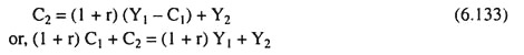
The budget constraint of the consumer states that the present value of consumption in the two period should be equal to that of the income of the two periods.
Therefore, the budget constraint is:
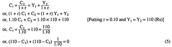
The relevant Lagrange function for constrained maximization of the (1) subject to (5) is
![]()
The 1st order conditions for constrained maximization of U is
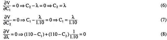
From (6) and (7), we have
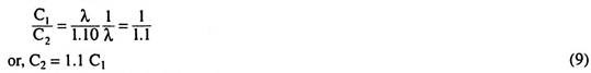
Putting the value of C2 in (8), we have
(110 – C1) + (110 – 1.1 C1). 1/1.1 = 0
Or, 110 – C1 + 110/1.1 – C1 = 0
Or, 2C1 = 210
Or, C1 = 105 (Rs)
From (9) C2 = 1.1 x 105 = 115.5 (Rs).
Therefore, the optimal consumption levels in the two periods (1 and 2) are 105 (Rs) and 115.5 (Rs), respectively.
(ii) Since Y1 = 110 (Rs) and C1 = 105 (Rs), the consumer lends in period 1 an amount = 110 – 105 = 5 (Rs)
In period 2, this amount accumulates to 5 x 1.1 = 5.5 (Rs). Therefore, the consumer borrows Rs 5.5 in period 2.