Income Consumption Curve: With Diagram | Indifference Curve | Economics

In this article we will discuss about the properties of an income consumption curve in different situations, with the help of suitable diagrams.

With a given money income to spend on goods, given prices of the two goods and given an indifference map (which portrays given tastes and preferences of the consumers), the consumer will be in equilibrium at, point in an indifference map.

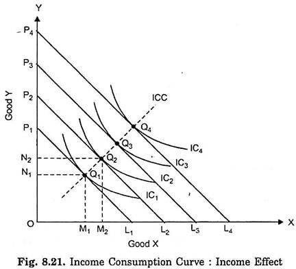
We are now interested in knowing how the consumer will react in regard to his purchases of the goods when his money income changes, prices of the goods and his tastes and preferences remaining un­changed. Income effect shows this reaction of the consumer. Thus, the income effect means the change in consumer’s purchases of the goods as a result of a change in his money income. Income effect is illustrated in Fig. 8.21.

With given prices and a given money income as indicated by the budget line P₁L₁, the consumer is initially in equilibrium at Q₁ on the indifference curve IC₁ and is having OM₁ of X and ON, of Y. Now suppose that income of the consumer increases. With his increased income, he Good X would be able to purchase larger quantities of both the goods.

As a result, budget line will shift upward and will be parallel to the original budget line P₁L₂. Let us assume that the consumer’s money income increases by such an amount that the new budget line is P₂L₂ (consumer’s income has increased by L₁L₂ in terms of X or P₁P₂ in terms of Y). With budget line PA, the consumer is in equilibrium at Q₂ on indifference curves IC₂ and is buying OM₂ of X and ON₂ of Y.

Thus, as a result of the increase in his income the consumer buys more quantity of both the goods. Since he is on the higher indifference curve IC₂he will be better off than before i.e., his satisfaction will increase. If his income increases further so that the budget line shifts to P₃L₃, the consumer is in equilibrium at Q₃ on indifference curve IC₃ and is having greater quantity of both the goods than at Q₂.

Conse­quently, his satisfaction further increases. In Fig. 8.21 the consumer’s equilibrium is shown at a still further higher level of income and it will be seen that the consumer is in equilib­rium at Q₄ on indifference curves IC₄ when the budget line shifts to P₄L₄. As the consumer’s income increases, he switches to higher indifference curves and as a consequence enjoys higher levels of satisfaction.

If now various points Q₁, Q₂, Q₃ and Q₄ showing consumer’s equilibrium at various levels of income are connected together, we will get what is called Income Consumption Curve (ICC). Income consumption curve is thus the locus of equilibrium points at various levels of consumer’s income. Income consumption curve traces out the income effect on the quantity consumed of the goods. Income effect can either be positive or negative.

Income effect for a good is said to be positive when with the increase in income of the consumer, his consumption of the good also increases. This is the normal case. When the income effect of both the goods represented on the two axes of the figure is positive, the income consumption curve (ICC) will slope upward to the right as in Fig. 8.21. Only the upward-sloping income consumption curve can show rising consumption of the two goods as income increases.

However, for some goods, income effect is negative. Income effect for a good is said to be negative when with the increases in his income, the consumer reduces his consumption of the good. Such goods for which income effect is negative are called Inferior Goods. This is because the goods whose consumption falls as the income of the consumer rises are considered to be some way ‘inferior’ by the consumer and therefore he substitutes superior goods for them when his income rises.

When with the increase in his income, the consumer begins to consume superior goods, the consumption or quantity purchased by him of the inferior goods tails. When the people are poor, they cannot afford to buy the superior goods which are often more expensive. Hence as they become richer and can afford to buy more expensive goods they switch to the consumption of superior and better quality goods.

For instance, most of the people in India consider cheapest common food-grains such as maize, jawar, bajra, as inferior goods and therefore when their income rises, they shift to the consumption of superior varieties of food-grains like wheat and rice. Similarly, most of the Indian people regard Vanaspati Ghee to be inferior and therefore as they become richer, they reduce its consumption and use ‘Desi Ghee’ instead.

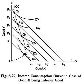
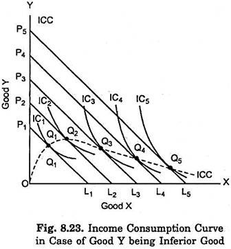
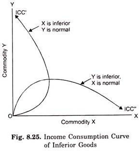
In case of inferior goods, indifference map would be such as to yield income consumption curve which either slopes backward (i.e., toward to the left) as in Fig. 8.22, or downward to the right as in Fig. 8.23. It would be noticed from the two figures that income effect becomes negative only after a point. It signifies that only at higher ranges of income, some goods become inferior goods and up to a point their consumption behaves like those of normal goods.

In Fig. 8.22 income consumption curve (ICC) slope backward (upward to the left) i.e., bends toward the Y-axis. This shows good X to be an inferior good, since beyond point Q_z, income effect is negative for good X and as a result its quantity demanded falls as income increases. In Fig. 8.23 income consumption curve (ICC) slopes downward to the right beyond point Q₂ i.e., bends towards the X-axis. This signifies that good Y is an inferior good because as beyond point Q₂, income effect is negative for good Y-and as a result its quantity demanded falls as income increases. It follows from above that the income consumption curve can have various possible shapes.

But normal goods can be either necessities or luxuries depending upon whether the quantities purchased of the goods by the consumers increase less than or more than propor­tionately to the increases in his income. If the quantity purchased of a commodity rises less than in proportion to increases in his income, the commodity is known as necessity.

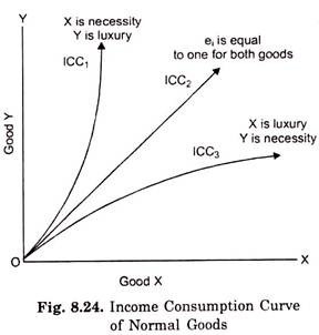
On the other hand, if the quantity purchased of a commodity increases more than proportionately to increases in his income, it is called a luxury. In Fig. 8.24, the slope of income consumption curve ICC₁ is increasing which implies that the quantity purchased of the commodity X increases less than proportionately to the increases in income. Therefore, in this case of ICC₁, good X is a necessity and good Y is luxury.

On the other hand, the slope of income consumption curve ICC₃ is decreasing which implies that the quantity purchased of good X increases more than proportionately to increases in income and therefore in this case good X is luxury and good Y is necessity. It will be seen from Fig. 8.24 that the income consump­tion curve ICC₂ is a linear curve passing through the origin which implies that the increases in the quantities purchased of both the goods are rising in proportion to income and there­fore neither good is a luxury or a necessity.

If the income effect is positive for both the goods X and Y, the income consumption curve will slope upward to the right as in Fig. 8.21. But upward-sloping income consumption curves to the right for various goods may be of different slopes as shown in Fig. 8.24 in which income consumption curves, with varying slopes, are all sloping upward and therefore indi­cate both goods to be normal goods having positive income effect.

If the income effect is negative, income consumption curve will slope backward to the left as ICC’ in Fig. 8.25 if good X happens to be an inferior good and income consumption curve will bend towards Y- axis if good Y happens to be an inferior good. In Figs. 8.24 and 8.25, various possible shapes which income consumption curve can take are shown bereft of indifference curves and budget lines which yield them. It may however be pointed out that given an indifference map and a set of budget lines there will be one income consumption curve.

A noteworthy point is that it is not the indifference curves which explain why a good happens to be an inferior good. In other words, indifference curves do not explain why income effect for a good is negative. Indifference curves only describe or illustrate the inferior-good phenomenon.