Total Demand and Supply for Money (With Diagram)

Read this article to learn about the total demand and supply for money in the rate of interest.

Total Demand for Money:

All the three motives give us the total demand for money (M₁ + M₂). The liquidity preference (demand for money) on account of transaction motive and precautionary motive is more or less stable and is almost interest-inelastic (except when interest rate is very high).

On the other hand, holdings on account of speculative motive are specially sensitive to changes in the rate of interest. If the total supply of money is represented by M, we may refer to the part of M held for transactions and precautionary motives as M₁ and to that part held for speculative motive as M₂ so that M – M₁ + M₂. Sometimes, money held under M₂ (transaction and precautionary motives) is termed as active balances or active money, whereas money held under M₂ (speculative motive) is termed as idle money or passive balances.

Since the amount of money held under M₁ depends upon income, it is expressed as M₁ – ƒ (Y) or M₁ = L₁ (Y). Similarly, M₂ = ƒ(r) or M₂ = L₂ (r). Therefore, the equation M = M₁ + M₂ may he written as (M) = L₁(Y) + L₂ (r). Thus, we find that given the supply of money (M) the rate of interest is determined by the liquidity preference (M₁ + M₂) and only that rate of interest will prevail which brings its (money’s) liquidity in equilibrium with the supply of money.

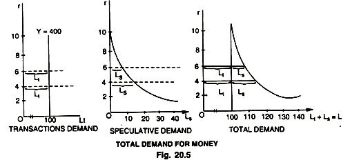
This figure shows the total demand for money, combining the equation L₃ = k(Y), which includes precautionary demand (L_p) also and the equation L_e = I(r), we now have an equation for the total demand for money:

L_t + L_s = k (K) + l(r)

We know from k what L_t will be for each level of Y and we know from I what L_s will be for each level of r. As such, we know from k and I what the total demand for money will be for every possible combination of Y and r. This is shown in the Fig. 20.5, in which part (A) shows the L_t for money as Rs. 100 crore when the level of income is Rs. 400 crore (assuming that k is 1/4). Part B shows the speculative demand for money (L_s) as an inverse function of the rate of interest. Part C shows the total demand for money or the sum of L_t and L_s. For example, at an income level of Rs. 400 crore and an interest rate of 4%, total demand for money is Rs. 110 crore, at the same income level but with an interest rate of 6%, total demand for money is Rs. 105 crore.

Supply of and Demand for Money:

By supply of money, we simply mean the sum total of currency and bank deposits held by the non-bank public. The monetary authority is responsible for determining the supply of money in an economy. It is, therefore, clear that the supply of the money is exogenously determined by the monetary authority and is not responsive to changes in the rate of interest. In other words, money supply curve is completely interest inelastic (that is, in fact, the position of Keynes and it is assumed as such).

The curve of money supply is, therefore, vertical. In the short run, the monetary authority permits the supply of money to increase or decrease. According to Keynes, the demand for money (liquidity preference) together with the supply of money, determines the rate of interest and hence the volume of investment and employment. The essence of Keynes’ theory of liquidity preference is that the quantity of money, along with the state of liquidity preference determines the rate of interest.

If people desire to hold more money, the monetary authority (Central Bank) alone can increase the supply of money. If the quantity of money is increased just in the same proportion as the increase in liquidity preference, the rate of interest will not rise, as it will when the quantity of money remains the same and the liquidity preference increases.

We have known that the rate of interest, being a monetary phenomenon, is determined by the demand for and supply of money. The demand for money comes from liquidity preference. The supply of money is determined by the Central Bank. It may be noted that the supply of money is different from the supply of commodities, the former being a stock and the latter a flow. Money is not continuously produced and simultaneously consumed as happens in case of commodities.

The supply of money can be controlled by the monetary authorities (Central Bank) and is more or less fixed. The monetary authorities can influence the rate of interest by increasing the supply of money (other things remaining the same), whereas they have no control over the liquidity preference of the people. Thus, the demand for liquidity, together with the supply of money, determines the interest rate.

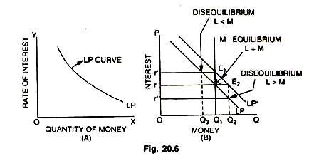
The relationship between the rate of interest, the quantity of money and liquidity preference (liquidity function) is shown in the Fig. 20.6:

In Fig. 20.6 (A), LP is the liquidity preference curve. It declines towards the right as the quantity of money increases. Given the level of income, the demand for money varies with the interest rate. In other words, liquidity preference is a function of the interest rate, increasing as the interest rate falls and decreasing as the interest rate rises. It is just like a demand curve, rate of interest being the price.

The reasons for this inverse relation between liquidity preference and the interest rate is that at a lower rate of interest, people find it more profitable to hold their savings in the form of cash balance (higher liquidity preferences) than at a higher rate of interest. That is why LP curve slopes downwards to the right. It is clear from the diagram that larger quantities of money are associated with lower rates of interest as long as the liquidity preference schedule remains unchanged.

(i) In Fig, 20.6 (B), LP is the liquidity preference curve (demand for money) which slopes downwards to the right showing that at a lower interest rate more money will be held.

(ii) The Q₁M curve shows the total amount of money which is assumed to be more or less fixed and inelastic with respect to interest rate (since it is fixed, the curve Q₁M is vertically straight).

(iii) At or rate of interest, the amount of money people wish to hold OQ₁ (liquidity preference) and the amount of money in existence OQ₁ coincide and the rate of interest is determined at KQ₁ i.e. where the demand for money (LP) is just equal to the supply of money. KQ₁ is called the equilibrium rate of interest, i.e. people have no desire to increase or decrease the stock of money by lending or investing, i.e., L = M.

(iv) At higher rate of interest Or” people would hold less money (OQ₃) and lend or invest the rest (Q₃Q₁). Thus, at a higher rate people’s liquidity preference is low because they gain more by lending or investing, i.e., L < M.

(v) On the other hand, when the rate of interest falls to Or”, people’s liquidity preference would increase from OQ₁ to OQ₂, (i.e., by O₁Q₂) because they lose more by lending or investing, i.e., L > M.

(vi) Further, when the LP curve shifts (rises) from LP to LP'(quantity of money remaining the same), the rate of interest also rises to E₁Q₁ from KQ₁.

(vii) Moreover, when the liquidity preference remaining the same (LP) but the quantity of money increases from OQ₁ to OQ₂, the rate of interest will fall from Or to Or”.