Top 5 Theories of Demand for Money

Here we detail about the top five theories of demand for money.

The theories are: (1) Fisher’s Transactions Approach, (2) Keynes’ Theory, (3) Tobin Portfolio Approach, (4) Boumol’s Inventory Approach, and (5) Friedman’s Theory.

Theory 1# Fisher’s Transactions Approach to Demand for Money:

In his theory of demand for money Fisher and other classical economists laid stress on the medium of exchange function of money, that is, money as a means of buying goods and services. All transactions involving purchase of goods, services, raw materials, assets require payment of money as value of the transaction made.

If accounting identity, namely value paid must equal value received is to occur, value of goods, services and assets sold must be equal to the value of money paid for them. Thus, in any given period, the value of all goods, services or assets sold must equal to the number of transactions 7 made multiplied by the average price of these transactions. Thus, the total value of transactions made is equal to PT.

On the other hand, because value paid is identically equal to the value of money flow used for buying goods, services and assets, the value of money flow is equal to the nominal quantity of money supply M multiplied by the average number of times the quantity of money in circulation is used or exchanged for transaction purposes. The average number of times a unit of money is used for transactions of goods, services and assets is called transactions velocity of circulation and is denoted by V.

Symbolically, Fisher’s equation of exchange is written as under:

MV = PT …(1)

Where, M = the quantity of money in circulation

V = transactions velocity of circulation

P = Average price

T = the total number of transactions.

The above equation (1) is an identity, that is true by definition. However by taking some assumptions about the variables V and T, Fisher transformed the above identity into a theory of demand for money.

According to Fisher, the nominal quantity of money M is fixed by the Central Bank of a country (note that Reserve Bank of India is the Central Bank of India) and is therefore treated as an exogenous variable which is assumed to be a given quantity in a particular period of time.

Further, the number of transactions in a period is a function of national income; the greater the national income, the larger the number of transactions required to be made. Further, since Fisher assumed that full employment of resources prevailed in the economy, the level of national income is determined by the amount of the fully employed resources.

Thus, with the assumption of full employment of resources, the volume of transactions T is fixed in the short run. But most important assumption which makes Fisher’s equation of exchange as a theory of demand for money is that velocity of circulation (V) remains constant and is independent of M, P and T.

This is because he thought that velocity of circulation of money (V) is determined by institutional and technological factors involved in the transactions process. Since these institutional and technological factors do not vary much in the short run, the transactions velocity of circulation of money (V) was assumed to be constant.

As we know that for money market to be in equilibrium, nominal quantity of money supply must be equal to the nominal quantity of money demand.

In other words, for money market to be in equilibrium:

M_s = M_d

where M_s is fixed by the Central Bank of a country.

With the above assumptions, Fisher’s equation of exchange in (1) above can be rewritten as

M_d = PT/V

or M_d = 1/V. PT …(2)

Thus, according to Fisher’s transactions approach, demand for money depends on the following three factors:

(1) The number of transactions (T)

(2) The average price of transactions (P)

(3) The transaction velocity of circulation of money

It has been pointed out that Fisher’s transactions approach represents some kind of a mechanical relation between demand for money (M_d) and the total value of transactions (PT). Thus Prof. Suraj Bhan Gupta says that in Fisher’s approach the relation between demand for money M_d and the value of transactions (PT) “betrays some kind of a mechanical relation between it (i.e. PT) and M_d as PT represents the total amount of work to be done by money as a medium of exchange. This makes demand for money (M_d) a technical requirement and not a behavioural function”.

In Fisher’s transactions approach to demand for money some serious problems are faced when it is used for empirical research. First, in Fisher’s transactions approach, not only transactions involving current production of goods and services are included but also those which arise in sales and purchase of capital assets such as securities, shares, land etc. Due to frequent changes in the values of these capital assets, it is not appropriate to assume that T will remain constant even if Y is taken to be constant due to full-employment assumption.

The second problem which is faced in Fisher’s approach is that it is difficult to define and determine a general price level that covers not only goods and services currently produced but also capital assets just mentioned above.

The Cambridge Cash Balance Theory of Demand for Money:

Cambridge Cash Balance theory of demand for money was put forward by Cambridge economists, Marshall and Pigou. This Cash Balance theory of demand for money differs from Fisher’s transactions approach in that it places emphasis on the function of money as a store of value or wealth instead of Fisher’s emphasis on the use of money as a medium of exchange.

It is worth noting that the exchange function of money eliminates the need to barter and solves the problem of double coincidence of wants faced in the barter system. On the other hand, the function of money as a store of value lays stress on holding money as a general purchasing power by individuals over a period of time between the sale of a good or service and subsequent purchase of a good or service at a later date.

Marshall and Pigou focused their analysis on the factors that determine individual demand for holding cash balances. Although they recognized that current interest rate, wealth owned by the individuals, expectations of future prices and future rate of interest determine the demand for money, they however believed that changes in these factors remain constant or they are proportional to changes in individuals’ income.

Thus, they put forward a view that individual’s demand for cash balances (i.e. nominal money balances) is proportional to the nominal income (i.e. money income).

Thus, according to their approach, aggregate demand for money can be expressed as:

M_d = kPY

Where, Y = real national income

P = average price level of currently produced goods and services

PY = nominal income

k = proportion of nominal income (PY) that people want to hold as cash balances

Cambridge Cash balance approach to demand for money is illustrated in Fig. 15.1 where on the X-axis we measure nominal national income (PY) and on the F-axis the demand for money (M_d). It will be seen from Fig. 15.1 that demand for money (M_d) in this Cambridge Cash Balance Approach

is a linear function of nominal income. The slope of the function is equal to k, that is, k = M_d/P_y .Thus important feature of Cash balance approach is that it makes the demand for money as function of money income alone.

A merit of this formulation is that it makes the relation between demand for money and income as behavioural in sharp contrast to Fisher’s approach in which demand for money was related to total transactions in a mechanical manner.

Although, Cambridge economists recognized the role of other factors such as rate of interest, wealth as the factors which play a part in the determination of demand for money but these factors were not systematically and formally incorporated into their analysis of demand for money.

In their approach, these other factors determine the proportionality factor k, that is, the proportion of money income that people want to hold in the form of money, i.e. cash balances. It was J.M. Keynes who later emphasized the role of these other factors such as rate of interest, expectations regarding future interest rate and prices and formally incorporated them explicitly in his analysis of demand for money.

Thus, Glahe rightly writes, “Cambridge approach is conceptually richer than the transactions approach, the former is incomplete because it does not formally incorporate the influence of economic variables just mentioned on the demand for cash balances… John Maynard Keynes first attempted to eliminate this shortcoming.”

Another important feature of Cambridge demand for money function is that the demand for money is proportional function of nominal income (M_d= kPY). Thus, it is proportional function of both price level (P) and real income (Y). This implies two things. First, income elasticity of demand for money is unity and, secondly, price elasticity of demand for money is also equal to unity so that any change in the price level causes equal proportionate change in the demand for money.

Criticism:

It has been pointed out by critics that other influences such as rate of interest, wealth, expectations regarding future prices have not been formally introduced into the Cambridge theory of the demand for cash balances. These other influences remain in the background of the theory. “It was left to Keynes, another Cambridge economist, to highlight the influence of the rate of interest on the demand for money and change the course of monetary theory.”

Another criticism leveled against this theory is that income elasticity of demand for money may well be different from unity. Cambridge economists did not provide any theoretical reason for its being equal to unity. Nor is there any empirical evidence supporting unitary income elasticity of demand for money.

Besides, price elasticity of demand is also not necessarily equal to unity. In fact, changes in the price level may cause non-proportional changes in the demand for money. However, these criticisms are against the mathematical formulation of cash balance approach, namely, M_d = kPY.

They do not deny the important relation between demand for money and the level of income. Empirical studies conducted so far point to a strong evidence that there is a significant and firm relation between demand for money and level of income.

Theory 2# Keynes’ Theory of Demand for Money:

In his well-known book, Keynes propounded a theory of demand for money which occupies an important place in his monetary theory. It is also worth noting that for demand for money to hold Keynes used the term what he called liquidity preference. How much of his income or resources will a person hold in the form of ready money (cash or non-interest-paying bank deposits) and how much will he part with or lend depends upon what Keynes calls his “liquidity preference.” Liquidity preference means the demand for money to hold or the desire of the public to hold cash.

Demand for Money or Motives for Liquidity Preference: Keynes’ Theory:

Liquidity preference of a particular individual depends upon several considerations. The question is: Why should the people hold their resources liquid or in the form of ready money when they can get interest by lending money or buying bonds?

The desire for liquidity arises because of three motives:

(i) The transactions motive,

(ii) The precautionary motive, and

(iii) The speculative motive.

1. The Transactions Demand for Money:

The transactions motive relates to the demand for money or the need for money balances for the current transactions of individuals and business firms. Individuals hold cash in order “to bridge the interval between the receipt of income and its expenditure”. In other words, people hold money or cash balances for transaction purposes, because receipt of money and payments do not coincide.

Most of the people receive their incomes weekly or monthly while the expenditure goes on day by day. A certain amount of ready money, therefore, is kept in hand to make current payments. This amount will depend upon the size of the individual’s income, the interval at which the income is received and the methods of payments prevailing in the society.

The businessmen and the entrepreneurs also have to keep a proportion of their resources in money form in order to meet daily needs of various kinds. They need money all the time in order to pay for raw materials and transport, to pay wages and salaries and to meet all other current expenses incurred by any business firm.

It is clear that the amount of money held under this business motive will depend to a very large extent on the turnover (i.e., the volume of trade of the firm in question). The larger the turnover, the larger, in general, will be the amount of money needed to cover current expenses. It is worth noting that money demand for transactions motive arises primarily because of the use of money as a medium of exchange (i.e. means of payment).

Since the transactions demand for money arises because individuals have to incur expenditure on goods and services during the receipt of income and its use of payment for goods and services, money held for this motive depends upon the level of income of an individual.

A poor man will hold less money for transactions motive as he spends less because of his small income. On the other hand, a rich man will tend to hold more money for transactions motive as his expenditure will be relatively greater

The demand for money is a demand for real cash balances because people hold money for the purpose of buying goods and services. The higher the price level, the more money balances a person has to hold in order to purchase a given quantity of goods. If the price level doubles, then the individual has to keep twice the amount of money balances in order to be able to buy the same quantity of goods. Thus the demand for money balances is demand for real rather than nominal balances.

According to Keynes, the transactions demand for money depends only on the real income and is not influenced by the rate of interest. However, in recent years, it has been observed empirically and also according to the theories of Tobin and Baumol transactions demand for money also depends on the rate of interest.

This can be explained in terms of opportunity cost of money holdings. Holding one’s asset in the form of money balances has an opportunity cost. The cost of holding money balances is the interest that is foregone by holding money balances rather than other assets. The higher the interest rate, the greater the opportunity cost of holding money rather than non-money assets.

Individuals and business firms economies on their holding of money balances by carefully managing their money balances through transfer of money into bonds or short-term income yielding non-money assets. Thus, at higher interest rates, individuals and business firms will keep less money holdings at each level of income.

2. Precautionary Demand for Money:

Precautionary motive for holding money refers to the desire of the people to hold cash balances for unforeseen contingencies. People hold a certain amount of money to provide for the danger of unemployment, sickness, accidents, and the other uncertain perils. The amount of money demanded for this motive will depend on the psychology of the individual and the conditions in which he lives.

3. Speculative Demand for Money:

The speculative motive of the people relates to the desire to hold one’s resources in liquid form in order to take advantage of market movements regarding the future changes in the rate of interest (or bond prices). The notion of holding money for speculative motive was a new and revolutionary Keynesian idea. Money held under the speculative motive serves as a store of value as money held under the precautionary motive does. But it is a store of money meant for a different purpose.

The cash held under this motive is used to make speculative gains by dealing in bonds whose prices fluctuate. If bond prices are expected to rise which, in other words, means that the rate of interest is expected to fall, businessmen will buy bonds to sell when their prices actually rise. If, however, bond prices are expected to fall, i.e., the rate of interest is expected to rise, businessmen will sell bonds to avoid capital losses.

Nothing is certain in the dynamic world, where guesses about the future course of events are made on precarious basis, businessmen keep cash to speculate on the probable future changes in bond prices (or the rate of interest) with a view to making profits.

Given the expectations about the changes in the rate of interest in future, less money will be held under the speculative motive at a higher current rate of interest and more money will be held under this motive at a lower current rate of interest.

The reason for this inverse correlation between money held for speculative motive and the prevailing rate of interest is that at a lower rate of interest less is lost by not lending money or investing it, that is, by holding on to money, while at a higher current rate of interest holders of cash balance would lose more by not lending or investing.

Thus the demand for money under speculative motive is a function of the current rate of interest, increasing as the interest rate falls and decreasing as the interest rate rises. Thus, demand for money under this motive is a decreasing function of the rate of interest. This is shown in Fig. 15.2. Along X-axis we represent the speculative demand for money and along the y-axis the current rate of interest.

The liquidity preference curve LP is downward sloping towards the right signifying that the higher the rate of interest, the lower the demand for money for speculative
motive, and vice versa. Thus at the high current rate of interest Or, a very small amount OM is held for speculative motive.

This is because at a high current rate of interest more money would have been lent out or used for buying bonds and therefore less money would be kept as inactive balances. If the rate of interest falls to Or’, then a greater amount of money OM is held under speculative motive. With the further fall in the rate -of interest to Or’, money held under speculative motive increases to OM.

Liquidity Trap:

It will be seen from Fig. 15.2 that the liquidity preference curve LP becomes quite flat i.e., perfectly elastic at a very low rate of interest; it is horizontal line beyond point E” towards the right. This perfectly elastic portion of liquidity preference curve indicates the position of absolute liquidity preference of the people. That is, at a very low rate of interest people will hold with them as inactive balances any amount of money they come to have.

This portion of liquidity preference curve with absolute liquidity preference is called liquidity trap by the economists because expansion in money supply gets trapped in the sphere of liquidity trap and therefore cannot affect rate of interest and therefore the level of investment. According to Keynes, it is because of the existence of liquidity trap that monetary policy becomes ineffective to tide over economic depression.

But the demand for money to satisfy the speculative motive does not depend so much upon what the current rate of interest is, as on expectations about changes in the rate of interest. If there is a change in the expectations regarding the future rate of interest, the whole curve of demand for money or liquidity preference for speculative motive will change accordingly.

Thus, if the public on balance expect the rate of interest to be higher (i.e., bond prices to be lower) in the future than had been previously supposed, the speculative demand for money will increase and the whole liquidity preference curve for speculative motive will shift upward.

Aggregate Demand for Money: Keynes’ View:

If the total demand of money is represented by M_d we may refer to that part of M held for transactions and precautionary motive as M₁ and to that part held for the speculative motive as M₂. Thus M_d= M₁ + M₂. According to Keynes, the money held under the transactions and precautionary motives, i.e., M₁, is completely interest-inelastic unless the interest rate is very high.

The amount of money held as M₁, that is, for transactions and precautionary motives, is mainly a function of the size of income and business transactions together with the contingencies growing out of the conduct of personal and business affairs.

We can write this in a functional form as follows:

M₁ = L₁(Y) …(i)

where Y stands for income, L₁ for demand function, and M₁ for money demanded or held under the transactions and precautionary motives. The above function implies that money held under the transactions and precautionary motives is a function of income.

On the other hand, according to Keynes, money demanded for speculative motive, i.e., M₂ as explained above, is primarily a function of the rate of interest.

This can be written as:

M₂ = L₂(r) …(ii)

Where r stands for the rate of interest, L₂ for demand function for speculative motive.

Since total demand of money M_d = M₁ + M₂, we get from (i) and (ii) above

M_d = L₁(Y) + L₂(r)

Thus, according to Keynes’ theory of total demand for money is an additive demand function with two separate components. The one component, L₁(Y) represents the transactions demand for money arising out of transactions and precautionary motives is an increasing function of the level of money income. The second component of the demand for money, that is, L₂(r) represents the speculative demand for money, which depends upon rate of interest, is a decreasing function of the rate of interest.

Critique of Keynes’ Theory:

By introducing speculative demand for money, Keynes made a significant departure from the classical theory of money demand which emphasized only the transactions demand for money. However, as seen above, Keynes’ theory of speculative demand for money has been challenged.

The main drawback of Keynes’ speculative demand for money is that it visualizes that people hold their assets in either all money or all bonds. This seems quite unrealistic as individuals hold their financial wealth in some combination of both money and bonds. This gave rise to portfolio approach to demand for money put forward by Tobin, Baumol and Friedman.

The portfolio of wealth consists of money, interest-bearing bonds, shares, physical assets etc. Further, while according to Keynes’ theory, demand for money for transaction purposes is insensitive to interest rate, the modern theories of money demand put forward by Baumol and Tobin show that money held for transaction purposes is interest elastic.

Further, Keynes’ additive form of demand for money function, namely, M_d= L_X(Y) + L₂ (r) has now been rejected by the modem economists. It has been pointed out that money represents a single asset, and not the several ones. There may be more than one motive to hold money but the same units of money can serve several motives. Therefore, the demand for money cannot be divided into two or more different departments independent of each other.

Further, as has been argued by Tobin and Baumol, the transactions demand for money also depends upon the rate of interest. Others have explained that speculative demand for money is an increasing function of the total assets or wealth. If income is taken as a proxy for total wealth then even speculative demand for money will depend upon the size of income, apart from the rate of interest.

In view of all these arguments, the Keynesian total demand for money function is written in the following modified form:

M_d = L(Y,r)

where it is conceived that demand for money function (M_d) is increasing function of the level of income, it is a decreasing function of the rate of interest. The presentation of the demand for money function in the above revised and modified form, M_d = L (Y, r) has been a highly significant development in monetary theory.

Theory 3# Tobin’s Portfolio Approach to Demand for Money:

American economist James Tobin, in his important contribution, explained that rational behaviour on the part of the individuals is that they should keep a portfolio of assets which consists of both bonds and money. In his analysis he makes a valid assumption that people prefer more wealth to less. According to him, an investor is faced with a problem of what proportion of his portfolio of financial assets he should keep in the form of money (which earns no interest) and interest-bearing bonds.

The portfolio of individuals may also consist of more risky assets such as shares. According to Tobin, faced with various safe and risky assets, individuals diversify their portfolio by holding a balanced combination of safe and risky assets. He points out that individual’s behaviour shows risk aversion. That is, they prefer less risk to more risk at a given rate of return. In Keynes’ analysis an individual holds his wealth in either all money or all bonds depending upon his estimate of the future rate of interest. But, according to Tobin, individuals are uncertain about future rate of interest.

If a wealth holder chooses to hold a greater proportion of risky assets such as bonds in his portfolio, he will be earning a high average return but will bear a higher degree of risk. Tobin argues that a risk averter will not opt for such a portfolio with all risky bonds or a greater proportion of them.

On the other hand, a person who, in his portfolio of wealth, holds only safe and riskless assets such as money (in the form of currency and demand deposits in banks) he will be taking almost zero risk but will also be having no return and as a result there will be no growth of his wealth. Therefore, people generally prefer a mixed diversified portfolio of money, bonds and shares, with each person opting for a little different balance between riskiness and return.

It is important to note that a person will be unwilling to hold all risky assets such as bonds unless he obtains a higher average return on them. In view of the desire of individuals to have both safety and reasonable return, they strike a balance between them and hold a mixed and balanced portfolio consisting of money (which is a safe and riskless asset) and risky assets such as bonds and shares though this balance or mix varies between various individuals depending on their attitude towards risk and hence their trade-off between risk and return.

Tobin’s Liquidity Preference Function:

Tobin derived his liquidity preference function depicting relationship between rate of interest and demand for money (that is, preference for holding wealth in money form which is a safe and “riskless” asset. He argues that with the increase in the rate of interest {i.e. rate of return on bonds), wealth holders will be generally attracted to hold a greater fraction of their wealth in bonds and thus reduce their holding of money.

That is, at a higher rate of interest, their demand for holding money (i.e., liquidity) will be less and therefore they will hold more bonds in their portfolio. On the other hand, at a lower rate of interest they will hold more money and less bonds in their portfolio. This means, like Keynes’ speculative demand for money, in Tobin’s portfolio approach demand function for money as an asset (i.e. his liquidity preference function curve) slopes downwards as is shown in Fig. 15.3, where on the horizontal axis asset demand for money is shown.

This downward-sloping liquidity preference function curve shows that the asset demand for money in the portfolio increases as the rate of interest on bonds falls. In this way Tobin derives the aggregate liquidity preference curve by determining the effects of changes in interest rate on the asset demand for money in the portfolio of individuals. Tobin’s liquidity preference theory has been found to be true by the empirical studies conducted to measure interest elasticity of the demand for money.

As shown by Tobin through his portfolio approach, these empirical studies reveal that aggregate liquidity preference curve is negatively sloped. This means that most of the people in the economy have liquidity preference function similar to the one shown by curve M_d in Fig. 15.3.

Evaluation:

Tobin’s approach has done away with the limitation of Keynes’ theory of liquidity preference for speculative motive, namely, individuals hold their wealth in either all money or all bonds. Thus, Tobin’s approach, according to which individuals simultaneously hold both money and bonds but in different proportion at different rates of interest, yields a continuous liquidity preference curve.

Further, Tobin’s analysis of simultaneous holding of money and bonds is not based on the erroneous Keynes’ assumption that interest rate will move only in one direction but on a simple fact that individuals do not know with certainty which way the interest rate will change.

It is worth mentioning that Tobin’s portfolio approach, according to which liquidity preference (i.e. demand for money) is determined by the individual attitude towards risk, can be extended to the problem of asset choice when there are several alternative assets, not just two, of money and bonds.

Theory 4# Baumol’s Inventory Approach to Transactions Demand for Money:

Instead of Keynes’ speculative demand for money, Baumol concentrated on transactions demand for money and put forward a new approach to explain it. Baumol explains the transactions demand for money from the viewpoint of the inventory control or inventory management similar to the inventory management of goods and materials by business firms.

As businessmen keep inventories of goods and materials to facilitate transactions or exchange in the context of changes in demand for them, Baumol asserts that individuals also hold inventory of money because this facilitates transactions (i.e. purchases) of goods and services.

In view of the cost incurred on holding inventories of goods there is need for keeping optimal inventory of goods to reduce cost. Similarly, individuals have to keep optimum inventory of money for transactions purposes. Individuals also incur cost when they hold inventories of money for transaction purposes.

They incur cost on these inventories as they have to forgo interest which they could have earned if they had kept their wealth in saving deposits or fixed deposits or invested in bonds. This interest income forgone is the cost of holding money for transaction purposes. In this way Baumol and Tobin emphasised that transaction demand for money is not independent of the rate of interest.

It may be noted that by money we mean currency and demand deposits which are quite safe and riskless but carry no interest. On the other hand, bonds yield interest or return but are risky and may involve capital loss if wealth holders invest in them. However, saving deposits in banks, according to Baumol, are quite free from risk and also yield some interest.

Therefore, Baumol asks the question why an individual holds money (i.e. currency and demand deposits) instead of keeping his wealth in saving deposits which are quite safe and earn some interest as well. According to him, it is for convenience and capability of it being easily used for transactions of goods that people hold money with them in preference to the saving deposits.

Unlike Keynes both Baumol and Tobin argue that transactions demand for money depends on the rate of interest. People hold money for transaction purposes “to bridge the gap between the receipt of income and its spending.” As interest rate on saving deposits goes up people will tend to shift a part of their money holdings to the interest-bearing saving deposits.

Individuals compare the costs and benefits of funds in the form of money with the interest- bearing saving deposits. According to Baumol, the cost which people incur when they hold funds in money is the opportunity cost of these funds, that is, interest income forgone by not putting them in saving deposits.

Baumol’s Analysis of Transactions Demand:

Baumol analyses the transactions demand for money of an individual who receives income at a specified interval, say every month, and spends it gradually at a steady rate. This is illustrated in Fig. 15.4. It is assumed that individual is paid Rs. 12000 salary cheque on the first day of each month. Suppose he gets it cashed (i.e. converted into money) on the very first day and gradually spends it daily throughout the month (Rs. 400 per day) so that at the end of the month he is left with no money.

It can be easily seen that his average money holding in the month will be Rs. 12000/2 = Rs. 6000 (before 15th of a month he will be having more than Rs. 6,000 and after 15th day he will have less than Rs. 6,000). Average holding of money equal to Rs. 6,000 has been shown by the dotted line.

Now, the question arises whether it is the optimal strategy of managing money or what is called optimal cash management. The simple answer is no. This is because the individual is losing interest which he could have earned if he had deposited some funds in interest-bearing saving deposits instead of withdrawing all his salary in cash on the first day. He can manage his money balances so as to earn some interest income as well.

Suppose, instead of withdrawing his entire salary on the first day of a month, he withdraws only half of it (i.e. Rs. 6,000) in cash and deposits the remaining amount of Rs. 6,000 in saving account which gives him interest of 5 per cent, his expenditure per day remaining constant at Rs. 400. This is illustrated in Fig. 15.5.

It will be seen that his money holdings of Rs. 6,000 will be reduced to zero at the end of the 15th day of each month. Now, he can withdraw Rs. 6,000 on the morning of 16th of each month and then spends it gradually, at a steady rate of 400 per day for the next 15 days of a month. This is a better method of managing funds as he will be earning interest on Rs. 6,000 for 15 days in each month. Average money holdings in this money management scheme is Rs. 6000/2 = 3000.

Likewise, the individual may decide to withdraw Rs. 4,000 (i.e., 1/3rd of his salary) on the first day of each month and deposits Rs. 8,000 in the saving deposits. His Rs. 4,000 will be reduced to zero, as he spends his money on transactions (that is, buying of goods and services), at the end of the 10th day and on the morning of 11th of each month he again withdraws Rs. 4,000 to spend on goods and services till the end of the 20th day and on 21st day of the month he again withdraws Rs. 4,000 to spend steadily till the end of the month.

In this scheme on an average he will be holding Rs. 4000/2 =2000 and will be investing remaining funds in saving deposits and earn interest on them. Thus, in this scheme he will be earning more interest income.

Now, which scheme will he decide to adopt? It may be noted that investing in saving deposits and then withdrawing cash from it to meet the transactions demand involves cost also. Cost on brokerage fee is incurred when one invests in interest-bearing bonds and sells them.

Even in case of saving deposits, the asset which we are taking for illustration, one has to spend on transportation costs for making extra trips to the bank for withdrawing money from the Savings Account. Besides, one has to spend time in the waiting line in the bank to withdraw cash each time from the saving deposits.

Thus, the greater the number of times an individual makes trips to the bank for withdrawing money, the greater the broker’s fee he will incur. If he withdraws more cash, he will be avoiding some costs on account of brokerage fee. Thus, individual faces a trade-off problem; the greater the amount of pay cheque he withdraws in cash, less the cost on account of broker’s fee but the greater the opportunity cost of forgoing interest income.

The problem is therefore to determine an optimum amount of money to hold. Baumol has shown that optimal amount of money holding is determined by minimizing the cost of interest income forgone and broker s fee. Let us elaborate it further.

Let the size of the pay cheque (i.e. salary) be denoted by Y, the average amount of the cash he withdraws each time the individual goes to the bank by C, the number of times he goes to the bank to withdraw cash by T, broker’s fee which he has to bear each time he makes a trip to the bank by b. In the first scheme of money management when he gets his whole pay-cheque cashed on the first day of every month he incurs broker’s fee only once since he makes only a single trip to the bank. Thus

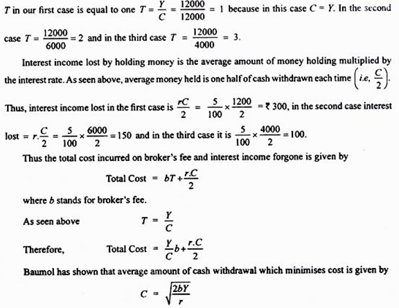
This means that average amount of cash withdrawal which minimizes cost is the square root of the two times broker’s fee multiplied by the size of individual’s income (Y) and divided by the interest rate. This is generally referred to as Square Root Rule. For this rule, it follows that a higher broker’s fee will raise the money holdings as it will discourage the individuals to make more trips to the bank.

On the other hand, a higher interest rate will induce them to reduce their money holdings for transaction purposes as they will be induced to keep more funds in saving deposits to earn higher interest income. That is, at a higher rate of interest transactions demand for money holdings will decline.

Keynes thought that transactions demand for money was independent of rate of interest. According to him, transactions demand for money depends on the level of income. However, Baumol and Tobin have shown that transactions demand for money is sensitive to rate of interest. Interest represents the opportunity cost of holding money instead of bonds, saving and fixed deposits.

The higher the rate of interest, the greater the opportunity cost of holding money (i.e. the greater the interest income forgone for holding money for transactions). Therefore, at a higher rate of interest people will try to economies the use of money and will demand less money for transactions.

At a lower interest rate on bonds, saving and fixed deposits, the opportunity cost of holding money will be less which will prompt people to hold more money for transactions. Therefore, according to Baumol and Tobin, transactions demand curve for money slopes downward as shown in Fig. 15.6. At higher interest rates, bonds, savings and fixed deposits are more attractive relative to money holding for transactions. Therefore, at higher interest rates people tend to hold less money for transaction purposes.

On the other hand, when the rates of interest are low, opportunity cost of holding money will be less and, as a consequence, people will hold more money for transactions. Therefore, the curve of transactions demand for money slopes downward.

It will be observed from the square root rule given above that transactions demand for money varies directly with the income (Y) of the individuals. Therefore, the higher the level of income, the greater the transactions demand for money at a given rate of interest. In Fig. 15.6. the three transactions demand curves for money M_d, M_d’ and M_d”, for three different income levels, Y₁, Y₂, Y₃are shown.

It will be known from the square root rule that optimum money holding for transactions will increase less than proportionately to the increase in income. Thus, transactions demand for money, according to Baumol and Tobin, is function of both rate of interest and the level of income.

M_td = f(r, y)

where M_td stands for transactions demand for money, r for rate of interest and Y for the level of income.

Theory 5# Friedman’s Theory of Demand for Money:

A noted monetarist economist Friedman put forward demand for money function which plays an important role in his restatement of the quantity theory of money and prices.  Friedman believes that money demand function is most important stable function of macroeconomics.

He treats money as one type of asset in which wealth holders can keep a part of their wealth. Business firms view money as a capital good or a factor of production which they combine with the services of other productive assets or labour to produce goods and services. Thus, according to Friedman, individuals hold money for the services it provides to them.

It may be noted that the service rendered by money is that it serves as a general purchasing power so that it can be conveniently used for buying goods and services. His approach to demand for money does not consider any motives for holding money, nor does it distinguish between speculative and transactions demand for money. Friedman considers the demand for money merely as an application of a general theory of demand for capital assets.

Like other capital assets, money also yields return and provides services. He analyses the various factors that determine the demand for money and from this analysis derives demand for money function. Note that the value of goods and services which money can buy represents the real yield on money.

Obviously, this real yield of money in terms of goods and services which it can purchase will depend on the price level of goods and services. Besides money, bonds are another type of asset in which people can hold their wealth. Bonds are securities which yield a stream of interest income, fixed in nominal terms. Yield on bond is the coupon rate of interest and also anticipated capital gain or loss due to expected changes in the market rate of interest.

Equities or Shares are another form of asset in which wealth can be held. The yield from equity is determined by the dividend rate, expected capital gain or loss and expected changes in the price level. The fourth form in which people can hold their wealth is the stock of producer and durable consumer commodities.

These commodities also yield a stream of income but in kind rather than in money. Thus, the basic yield from commodities is implicit one. However, Friedman also considers an explicit yield from commodities in the form of expected rate of change in their price per unit of time.

Friedman’s nominal demand function (M_d) for money can be written as:

M_d = f(W, h, r_m, r_b, r_e, P, ∆P/P, U)

As demand for real money balances is nominal demand for money divided by the price level, demand for real money balances can be written as:

M_d/P = f(W, h, r_m, r_b, r_e, P, ∆P/P, U)

where M_d stands for nominal demand for money and M_d/P for demand for real money balances, W stands for wealth of the individuals, h for the proportion of human wealth to the total wealth held by the individuals, r_m for rate of return or interest on money, r_b for rate of interest on bonds, r_e for rate of return on equities, P for the price level, ∆P/P for the change in price level (i.e. rate of inflation), and U for the institutional factors.

1. Wealth (W):

The major factor determining the demand for money is the wealth of the individual (W). In wealth Friedman includes not only non-human wealth such as bonds, shares, money which yield various rates of return but also human wealth or human capital. By human wealth Friedman means the value of an individual’s present and future earnings. Whereas non-human wealth can be easily converted into money, that is, can be made liquid.

Such substitution of human wealth is not easily possible. Thus human wealth represents illiquid component of wealth and, therefore, the proportion of human wealth to the non-human wealth has been included in the demand for money function as an independent variable.

Individual’s demand for money directly depends on his total wealth. Indeed, the total wealth of an individual represents an upper limit of holding money by an individual and is similar to the budget constraint of the consumer in the theory of demand. The greater the wealth of an individual, the more money he will demand for transactions and other purposes.

As a country becomes richer, its demand for money for transaction and other purposes will increase. Since as compared to non- human wealth, human wealth is much less liquid, Friedman has argued that as the proportion of human wealth in the total wealth increases, there will be a greater demand for money to make up for the illiquidity of human wealth.

2. Rates of Interest or Return (r_m, r_b, r_e):

Friedman considers three rates of interest, namely, r_m, r_b and r_e which determine the demand for money. r_m is the own rate of interest on money. Note that money kept in the form of currency and demand deposits does not earn any interest.

But money held as saving deposits and fixed deposits earns certain rates of interest and it is this rate of interest which is designated by r_m in the money demand function. Given the other rates of interest or return, the higher the own rate of interest, the greater the demand for money.

In deciding how large a part of his wealth to hold in the form of money the individual will compare the rate of interest on money with rates of interest (or return) on bonds and other assets. The opportunity cost of holding money is the interest or return given up by not holding these other forms of assets.

As rates of return on bond (r_b) and equities (r_e) rise, the opportunity cost of holding money will increase which will reduce the demand for money holdings. Thus, the demand for money is negatively related to the rate of interest (or return) on bonds, equities and other such non-money assets.

3. Price Level (P):

Price level also determines the demand for money balances. A higher price level means people will require a larger nominal money balance in order to do the same amount of transactions, that is, to purchase the same amount of goods and services.

If income (Y) is used as proxy for wealth (W) which, as stated above, is the most important determinant of demand for money, then nominal income is given by Y.P which becomes a crucial determinant of demand for money. Here Y stands for real income (i. e. in terms of goods and services) and P for price level.

As the price level goes up, the demand for money will rise and, on the other hand, if price level falls, the demand for money will decline. As a matter of fact, people adjust the nominal money balances (M) to achieve their desired level of real money balance (M/P).

4. The Expected Rate of Inflation (∆P/P):

If people expect a higher rate of inflation, they will reduce their demand for money holdings. This is because inflation reduces the value of their money balances in terms of its power to purchase goods and services.

If the rate of inflation exceeds the nominal rate of interest, there will be negative rate of return on money. Therefore, when people expect a higher rate of inflation they will tend to convert their money holdings into goods or other assets which are not affected by inflation.

On the other hand, if people expect a fall in the price level, their demand for money holdings will increase.

5. Institutional Factors (U):

Institutional factors such as mode of wage payments and bill payments also affect the demand for money. Several other factors which influence the overall economic environment affect the demand for money. For example, if recession or war is anticipated, the demand for money balances will increase.

Besides, instability in capital markets, which erodes the confidence of the people in making profits from investment in bonds and equity shares, will also raise the demand for money. Even political instability in the country influences the demand for money. To account for these institutional factors Friedman includes the variable U in his demand for money function.

Simplifying Friedman’s Demand for Money Function:

A major problem faced in using Friedman’s demand for money function has been that due to the non-existence of reliable data about the value of wealth (W), it is difficult to estimate the demand for money. To overcome this difficulty Friedman suggested that since the present value of wealth or W= Y_p/r (where Y_p is the permanent income and r is the rate of interest on money.), permanent income Y_p can be used as a proxy variable for wealth.

Incorporating this in Friedman’s demand for money function we have:

M_d = (Y_p, h, r_m, r_b, r_e, P, ∆P/P, U)

If we assume that no price change is anticipated and institutional factors such as h and U remain fixed in the short run and also all the three rates of interest return are clubbed into one, Friedman’s demand for money function is simplified to

M_d = f(Y_pr)