Relationship among AR, MR and Elasticity of Demand

Let us learn about the relationship between AR, MR and elasticity of demand.

1. Geometrical Method:

In Fig. 3.36. DT is the average revenue curve or the demand curve of a firm operating under imperfect competition. We know that elasticity of demand on the demand curve DT at point Q = QT/QD. A perpendicular QP is drawn to the vertical axis and another perpendicular QA has been drawn on the horizontal axis. MR curve bisects the perpendicular QP at point H.

Now, in triangles PDQ and AQT, we have

∟DPQ =  ∟QAT (right angles)

∟DQP = ∟QTA (corresponding angles)

and ∟PDQ =  ∟AQT

Thus triangles PDQ and AQT are equiangular. So, we can write

QT/QD = QA/PD

Again, in the triangles PDH and HQN, PH = HQ.

∟PHD = ∟QHN (vertically opposite angles)

∟DPH = ∟HQN (right angles)

Therefore, triangles PDH and HQN are congruent (i.e., equal in all respects). Therefore, DP = QN.

Thus elasticity of demand at point Q is

QT/QD = QA/PD = QA/QN

But, QN = QA – NA

.^.. QA/QN = QA/QA-NA

Hence, elasticity of demand at

Q =QA/QA-NA

It is clear from Fig. 3.36 that QA is the average revenue while NA is the marginal revenue for the output OA. Hence, elasticity at Q is

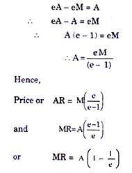
e = AR/AR – MR

or, e = A/A – M 

where A stands for average revenue and M for marginal revenue.

By cross-multiplication one gets

This formula helps us to find MR at any output from AR at the same output. Suppose, price of a product is Rs. 10. If elasticity of demand is equal to 2, then

MR = AR (1 – 1/e) = 10 (1- ½) = Rs.5

If elasticity of demand equals 1 then

MR = AR (1 – 1/e) = 10 = (1 – 1/1) = Rs. 0

If elasticity is equal to less than 1, say 1/2, then

MR = AR (1 – 1/e) = 10 (1 – 1/1/2) = Rs. -10

Thus, MR will be positive if the coefficient of elasticity of demand is elastic (i.e., e > 1). MR will be zero if elasticity is equal to one (i.e., e = 1), and MR will be negative if coefficient of elasticity is inelastic (i.e., e < 1).

2. Algebraic Method:

A mathematical method is also employed to describe the relationship among AR, MR and e.

Suppose, initial price and quantity are P and Q, respectively.

Thus,

TR₀ = P × Q

Now, let the price fall by ∆P and quantity rise by ∆Q. Now the total revenue will be

TR₁ = (P – ∆P). (Q + ∆Q)

∆TR = TR₁ – TR₀

= (P – ∆P) (Q + ∆Q) – P.Q

or ∆TR = PQ + P∆Q- Q∆P- ∆P∆Q – PQ

= P∆Q – Q∆P – ∆P∆Q

Ignoring ∆P∆Q as infinitesimally small, ∆TR = P∆Q – Q∆P.

MR is defined as the change in total revenue consequent upon a change in output, i.e.,

MR = ∆TR/∆Q = P∆Q – Q∆P/∆Q = P – Q∆P/∆Q

Now, we multiply this term by P/1, which does not change the equality.

Thus,

MR = P – (∆P/∆Q). (Q/P). (P/1)

Factoring out P we obtain

MR = P (1 – ∆P/∆Q. Q/P)= P (1 – 1/e)

[e = ∆Q/∆P. P/Q .^.. 1/e = ∆P/∆Q. Q/P]

MR = P (1 – 1/e)

Thus, we can say that (1) MR depends on (i) the price of the product, and (ii) elasticity of demand for the product, and (2) as the value of e rises, declines. If the value of e becomes infinite then

MR = P (1 – 1/e) = P (1 – 1/∞) = P (1 – 0) = P

Or, MR coincides with AR (or P). This happens under perfect competition.

The formula MR = P (1 – 1/e) enables us to derive price i.e., P = MR ÷ (1 – 1/e).

If MR is 2 and e is also 2, then

P = 2 ÷ (1 – 1/e) = 4