
The price elasticity of demand in the words of Marshall can be defined as, the elasticity of demand in a market is great or small according as the amount demanded increases much or little for a given fall in price and diminishes much or little for a given rise in price.
In this article we will discuss about:- 1. Definitions of Price Elasticity of Demand 2. Diagrammatic Representation of Price Elasticity 3. Types 4. Errors 5. Factors 6. Measurement 7. Formulas and 8. Examples.
Definitions of Price Elasticity of Demand:
Some of the important definitions of the price elasticity of demand, as given by different authors, are present below:
The price elasticity of demand in the words of Marshall can be defined as, the elasticity of demand in a market is great or small according as the amount demanded increases much or little for a given fall in price and diminishes much or little for a given rise in price.
ADVERTISEMENTS:
In the words of Gould and Lazear, the price elasticity of demand is the relative responsiveness of quantity demanded to changes in commodity price.
In the words of Meyers, the elasticity of demand is measure of the relative change in the amount purchased in response to relative change in the price on a demand curve.
Stonier and Hague defined it as, Elasticity of demand is a technical term used by economists to describe the degree of responsiveness of the demand for a goods to change in its price.
Mrs. J. Robinson wrote, the proportionate change in quantity demanded in response to a small change I price, divided by the proportionate change in price.
Sign of the Elasticity Estimate:
The price elasticity estimates always carry a negative sign because either ΔQ or ΔP will be negative due to inverse price-quantity relationship. However, the negative sign, which represents the direction of change, is ignored while analyzing the elasticity coefficient and only its numeric value is taken into consideration.
ADVERTISEMENTS:
The price elasticity of demand in the above mentioned example of cheese demand in India and England is estimated as – 0.5 in case of India but – 2.0 in case of England. If the negative sign is not ignored, the cheese demand will be analyzed as more elastic in India (–0.5) than that in England (–2.0).
However, ignoring the negative sign, which just indicate the inverse price- quantity relationship, we can argue that the cheese demand in England (2.0) is four times more responsive to a change in price than that in India (0.5). In other words, a 10% fall in price of cheese will result into a 5% increase in its demand in India but a 20% increase in England.
How a Situation is viewed:
Another important point with regard to elasticity of demand is that the estimate depends upon how to view a situation. We may read the situation as a fall in cheese price from Rs.10 to Rs.5 or an increase from Rs.5 to Rs.10 the estimate of price elasticity will be different in both cases. For England, the estimate will be – 2 when a fall in price is considered but only – 0.5 when an increase in price is considered in the same situation.
ADVERTISEMENTS:
The two estimates will present a radically different picture of demand responsiveness: highly elastic when a fall in price is considered and inelastic when an increase in price is considered in the same case. Such a situation of contrary results will be taken care of under the Arc method of measuring the elasticity.
Slope and Price Elasticity of Demand:
The elasticity of a demand is not the same as its slope. The slope (or 1/slope, i.e. the reciprocal of slope) is one of the two components of the elasticity and measured as ΔP/ΔQ. Its other component of price elasticity of demand is P/Q.
Therefore, elasticity of demand will differ even on a straight line demand curve which has the same slope at all its points since the P/Q will be different at each point.
So far slope is concerned, it can be stated that higher the slope of demand curve lesser will be the elasticity and vice versa, other things remaining the same.
Diagrammatic Representation of Price Elasticity:
In the figure 7.1. Ep is called the elasticity co-efficient or the coefficient of price elasticity of demand which is used to measure the responsiveness of market demand. Since the demand curve is downward sloping, either P change or Q change has to be negative. Thus, the ratio (Ep) is negative. This is why we have to put a negative sign to get a positive value of the coefficient.
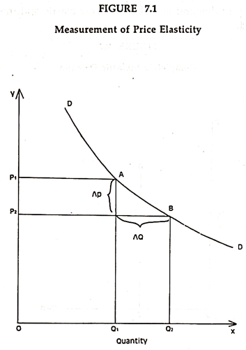
The elasticity of demand with regard to price of the commodity is always having a minus sign. This means that price and demand are inversely related. The negative sign is not ordinarily used in writing the price elasticity of demand. The negative sign is understood.
Types of Price Elasticity:
There are four types of elasticity of demand:
(1) Completely inelastic demand,
ADVERTISEMENTS:
(2) Perfectly elastic demand,
(3) Unitary elasticity of demand and
(4) Relatively elastic and inelastic demand.
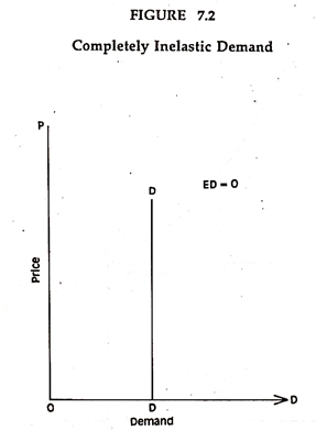
(1) Completely Inelastic Demand:
ADVERTISEMENTS:
In Figure 7.2 the straight line demand curve is parallel to the vertical axis that showing price. This means that whatever the changes in price may be, the amount demanded remain the same. The elasticity of demand is equal to zero.
(2) Perfectly Elastic Demand:
Perfectly elastic demand is one in which small change in price will cause an infinity large changed in demand (see Figure 7.3.). A small reduction in price lead to big change in demand. It is a straight line demand curve parallel to horizontal axis.
ADVERTISEMENTS:

(3) Unitary Elasticity of Demand:
A given parentage change in price lead to exactly the same percentage change in demand is the main theme of the unitary elasticity of demand.
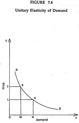
As shown in the Figure 7.4, the curve DD is known as constant-total-outlay curve. This figure depicts that the total expenditure is equal to the quantity demanded multiplied by price. When the price is OT, the demand is OM, then the total expenditure (i.e. OT x OM) is the area of the rectangle OMPT.
At OL, total expenditure is the area of rectangle ONKL. The total area of rectangle is always equal. Whenever a part or the whole of demand curve is of the shape of a rectangular hyperbola, its elasticity of demand on that part equals one.
ADVERTISEMENTS:
(4) Relatively Elastic and Inelastic Demand:
The demand curves which have elasticity between zero and infinity are called relatively elastic and inelastic demand. When the demand curve having higher value of elasticity it is called relatively elastic, and when the demand curve having lower value of elasticity, it is called the relatively inelastic.
Mistakes/Errors of Price Elasticity:
To call demand curve as elastic or inelastic is altogether wrong. Elasticity of demand is shown by a point on demand curve at different points and, therefore, they have different elasticities.
Without any thought about the definition of elasticity, steep sloped demand curves are called inelastic and the demand curves with gentle slope are referred to as elastic. The slope of the demand curve shows the ratio between the absolute change in price and the absolute change in demand.
Factors Determining Price Elasticity:
The following are the important factors that determine the price elasticity:
1. Availability of Substitutes:
ADVERTISEMENTS:
If a commodity has close substitutes, then the demand for the commodity will be quite price elastic. Ex. Coca cola, Gold Spot etc.
2. Nature of the Commodity:
Price Elasticity for necessaries is low while that of luxuries is quite high.
3. Number of Use of a Commodity:
The greater the number of uses the higher the price elasticity of demand and vice-versa.
4. Incomes of the Consumers:
ADVERTISEMENTS:
Price elasticity of demand of high income class for high quality is low but of poor class is very high.
5. Habitual Necessities:
Although prices of cigarettes etc., are rising, their demand has not diminished. It is price inelastic.
Methods of Measurement:
There are three important types of measurement of price elasticity, and they are:
(a) Percentage Method,
(b) Arc Method, and
ADVERTISEMENTS:
(c) Total Outlay Method.
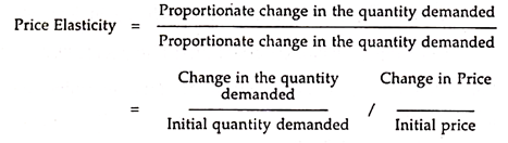
(a) The Percentage Method:
The formula for measuring the elasticity of demand under this method may be written as:
If the percentage change are known, than the numerical size of E (elasticity of demand) can be calculated. Suppose the price has fallen by 20% and the demand has expanded by 20% as a result of the fall in price.
The elasticity of demand is therefore:

When the demand change by the same percentage as the price elasticity is equal to one or unity.
If the percentage changes in demand are more than that in price, then elasticity is greater than one.
For Example:

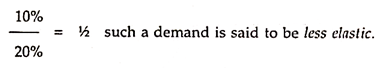
If the percentage change in demand is less than in price, then elasticity is less than one.
For Example:
(b) Arc Method:
The arc method of measurement of price elasticity is to use the average of the original price and the changed price, origin demand and changed demand. This is called Arc Elasticity of Demand (ED).

It gives more consistent measure than point ED.
We can illustrate the arc method of elasticity of demand as shown in the figure 7.5:
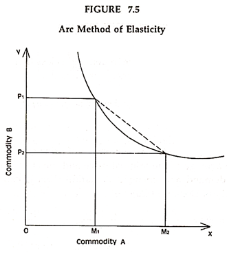
This can be used for a small change in price (Figure 7.5.). At OP1 and OP2 prices, the A commodity demanded at OM1 and OM2. The two points are of more distance so, it will not yield the correct measure of elasticity price. Because, the elasticity formula takes into consideration the straight line joining the two points rather than the arc is showing a lesser area than the triangle used for point-elasticity.
(c) Total Outlay Method:
Elasticity of Demand can be measured from the changes in the expenditure of consumers as price changes. Marshall was the major proponent of this method and he called it the Total Expenditure Method and Outlay Method.
The theory has following propositions:
1. Elasticity of Demand equal to one i.e. ED = 1. A small change in price leads to small purchase.
2. Elasticity of Demand greater than one i.e. ED > 1. A small fall in price leads to an increase in total outlay.
3. Elasticity of Demand lesser than one i.e. ED < 1. A small change in price leads to changes in total expenditure.
Diagrammatic Representation of Total Outlay Method:
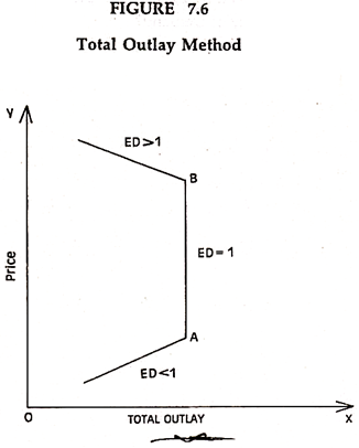
As the Figure 7.6 shows, change in price leads to change in the total outlay also. If price rises, total outlay also increase, elasticity is, then, less than one. In LA portion, both price and total outlay are raising, therefore, ED < 1. In AB portion of total expenditure curve, the total expenditure remains the same, while process are rising, then ED = 1. In BC portion price is rising but total expenditure is falling, then ED > 1.