Elasticity of Demand and Supply (With Diagram)

Read this article to learn about Elasticity of Demand and Supply: – 1. Subject Matter of Elasticity of Demand and Supply 2. Meaning of Price Elasticity of Demand 3. Different Kinds of Price Elasticities 4. Elasticity and Slope 5. Elasticity and Total Revenue/Total Expenditure 6. Determinants of Price Elasticity 7. Value of Elasticity 8. Arc Elasticity and others.

Elasticity of Demand and Supply # 1. Subject Matter:

Demand and Supply Theory is essential for an understanding of economics.

It has been argued that certain relationships exist between price and quantity demanded and supplied, other things remaining constant.

But if price changes, by how much does quantity demanded or supplied change? It could be that a large price increase/decrease will have little effect of quantity demanded or supplied.

On the other hand, a small price increase/decrease might result in a substantial change in demand or supply. Theoretically it is impossible to say exactly what will happen in cases like these. Each product may have a different price-quantity reaction. It is a matter for economists to collect evidence and calculate this relationship.

However, theoretical economists can provide a useful guidance for studying this relationship. Elasticity is a measure of the relationship between quantity demanded or supplied and another variable, such as price or income, which affects the quantity demanded or supplied.

Elasticity of Demand and Supply # 2. Meaning of Price Elasticity of Demand:

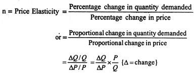
Price Elasticity of demand measures the degree of responsiveness of the quantity demanded of a commodity to change in its price. Thus its measure depends upon comparing the percentage change in the price with the resultant percentage change in the quantity demanded.

Exact formulations are as follows:

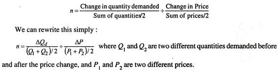
There is a slight problem with computation of percentage changes in this manner. We get different answers depending on whether we move up or down the demand curve. One way out of this difficulty is to take the average of two prices and the two quantities over the range we are considering and comparing the change of the average, instead of comparing it to the price or quantity at the start of the change.

The formula for calculating price elasticity of demand then becomes:

Elasticity of Demand and Supply # 3. Different Kinds of Price Elasticities:

We have different ranges of price elasticities, depending on whether a 1% change in price elicits more or less than a 1% change in quantity demanded.

a. Price-Elastic Demand:

If the price elasticity of demand is greater than one, we call this a price-elastic demand. A 1% change in price causes a response greater than 1% change in quantity demanded: ΔP < ΔQ.

b. Unitary Price Elasticity of Demand:

In this case, a 1% change in price causes a response of exactly 1% change in the quantity demanded.

When Area A = Area B, Rectangular Hyperbola! ΔP = AQ.

c. Price-Inelastic Demand:

Hence, a 1% change in price causes a response of less than 1% change in quantity demanded: ΔP > ΔQ.

Elasticity of Demand and Supply # 4. Elasticity and Slope:

Elasticity and Slope are not the same. We will demonstrate that along a linear demand curve (that is, a straight line with a constant slope) elasticity falls with price. As a matter of fact, the elasticity along a downward-sloping Straight line demand curve goes numerically from infinity to zero as we move down the curve.

We must, therefore, specify the price range when discussing price elasticity of demand, since most goods have ranges of both elasticity and inelasticity. The only time we can be sure of the elasticity of a straight line demand curve by looking at it is if it is either perfectly horizontal or perfectly vertical. The horizontal straight line demand curve has infinite elasticity at every quantity as given in Fig. 3.4(a).

The vertical demand curve has zero elasticity at every price as given in Fig. 3.4(b):

Extreme Elasticities:

In Fig. 3.4(a), we show complete responsiveness. At a price of 20p, consumers will demand an unlimited quantity of the commodity in question. In Fig. 3.4(b), we show complete price unresponsiveness. The demand curve is vertical at the quantity Q₁ unit. That means the price elasticity of demand is zero here. Consumers demand Q₁ units of this particular commodity — no matter what the price is.

Elasticity of Demand and Supply # 5. Elasticity and Total Revenue/Total Expenditure:

It is generally thought that the way to increase total receipts or total expenditure is to increase price per unit. But is this always the case? Is it possible that a rise in price per unit could lead to a decrease in total revenue? The real answers to these questions depend on the price elasticity of demand.

In Table 3.1, we show in column 1 price of petrol in pounds, in column (2) units demanded (per time period), in column (3) total revenues (P x Q) and in column (4) values of elasticity. Notice what happens to total revenue throughout the schedule.

They rise steadily as the price rises from £1 to £5 per unit; then, when the price rises further to £6 per unit, total revenue remains constant at £30. At prices higher than £6, total revenue actually falls as price is increased. So it is not safe to assume that a price increase is always the way to greater revenues.

Indeed, if prices are above £6 per unit in our example, total revenue can only be increased by cutting prices.

Here, in Table 3.1, we show the elastic, unit elastic and inelastic sections of the demand schedule according to whether a reduction in price increases total revenue, causes them to remain constant, or causes them to decrease. In Fig. 3.5, we show graphically what happens to total revenue in elastic, unit-elastic and inelastic part of the demand curve.

Hence, we have three relationships among the three types of price elasticity and total revenue:

a. Price-Elastic Demand:

A negative relationship exists between small changes in price and changes in total revenue. That is, if price is lowered, total revenue will rise when the firm faces price-elastic demand. And, if it raises price, total revenue will fall.

b. Unit Price-Elastic Demand:

Small changes in price do not change total revenue. In other words, when the firm is facing demand that is unit-elastic, if it increases price, total revenue will not change; if it decreases price, total revenue will not change either.

c. Price-Inelastic Demand:

A positive relationship between small changes in price and total revenue. That is, when the firm is facing demand that is price-inelastic, if it raises price, total revenue will go up; if it reduces price, total revenue will fall. We can see in Fig. 3.5 the areas in the demand curve that are elastic, unit-elastic and inelastic. For price rise from £1 to £5 per unit, total revenue rises from £10 to £30, as demand is price-inelastic.

When price changes from £5 to £6, however, total revenue remains constant; at £30, demand is unit-elastic. Finally, when price rises from £6 to £11, total revenue decreases from £30 to 0. Clearly, demand is price-elastic. This has been shown distinctly in Fig. 3.5.

The relationship between the price elasticity of demand and total revenue brings together some important microeconomic concepts. Total revenue is the product of price per unit times quantity of units sold (P x Q).

The theory of demand states that, along a given demand curve, price and quantity changes will move in opposite directions one increases and other decreases. Consequently, what happens to the product of price times quantity depends on which of the opposing changes exerts a greater force on total revenue. This is what price elasticity of demand is designed to measure responsiveness of quantity to a change in price.

The relationship between price elasticity of demand and total revenue is summarized:

Elasticity of Demand and Supply # 6. Determinants of Price Elasticity:

a. Ease of Substitution:

The greater the number of substitutes available for a product, the greater will be its elasticity of demand. For example, food as a whole has a very inelastic demand but when we consider any particular item of food we will find that the elasticity of demand is much greater. This is because, while we can find no substitute for food as a whole, we can, however, always find substitute for one type of food for another.

b. Number of Uses:

The greater the number of uses to which a commodity can be put, the greater is its elasticity of demand. For example, electricity has many uses — heating, lighting, cooking, etc. A rise in the price of electricity might cause people not only to economise in all these areas but also to substitute other fuels in some cases.

c. Proportion of Income Spent on the Product:

If the price of a packet of salt were to rise by 50%, for example from 20p to 30p, it would discourage very few people because it constitutes a very small proportion of their income. However, if the price of a car were to rise from £4,000 to £6,000, it would have an enormous effect on sales, even though it would be the same percentage increase.

The greater the proportion of income which the price of the product represents the greater its elasticity of demand will tend to be.

d. Time:

In general, elasticity of demand will tend to be greater in the long-run than in the short-run. The period of time we are considering plays an important role in shaping the demand curve. For example, if the price of meat rises disproportionately to other foods, eating habits cannot be changed immediately.

So, people will continue to demand the same amount of meat in the short-run. But, in the long-run, people will begin to seek substitutes. Whether or not this is a noticeable effect will depend upon whether or not consumers discover adequate substitutes. It may also be possible to obscure the opposite effect.

e. Durability:

The greater the durability of a product, the greater its elasticity of demand will tend to be. For example, if the price of potatoes rises, it is not possible to eat the same potatoes twice. However, if the price of furniture rises, we can make our existing furniture last longer.

f. Addiction:

Where a product is habit-forming, for example, cigarettes, this will tend to reduce its elasticity of demand.

g. The Price of Other Products:

We know that a rise in the price of a product will cause the demand for its substitutes to rise and the demand for its complements to fall. Thus, an increase (or decrease) of demand by a constant percentage leaves elasticity unchanged, but a rightward shift of the curve by a fixed amount reduces elasticity.

In both diagrams in Fig. 3.6, there has been an increase in demand which has moved the demand curve rightwards. In diagram 3.6(a), it can been seen that the shift of the whole curve to the right has reduced its elasticity. In Fig. 3.6(b), however, demand has increased by a constant percentage at every price, elasticity has remained constant.

(a) Elasticity decreases when the whole demand curve moves out wards.

(b) Elasticity remains unchanged when demand curve swivels.

Elasticity of Demand and Supply # 7. Value of Elasticity:

An increase (+) in price will cause a fall (-) in quantity and, conversely a decree (-) in the value of the answer must always be negative. The coefficient is expressed as S by putting a minus sign in front of the equation, thus: E_D = –

Elasticity of Demand and Supply # 8. Arc Elasticity:

It is an estimate of elasticity along a range of a demand curve.

It can be calculated for both linear and non-linear demand curves using the following formula:

Arc elasticity of demand:

In this formula P₁ and q₁ represent the original price and quantity, and P₂ and q₂ represent the new price and quantity.

Thus, (P₁ + P₂)/2 is a measure of the average price in the range along the demand curve and (q₁ + q₂) / 2 is the average quantity in this range.

Elasticity of Demand and Supply # 9. Short-Run and Long-Run:

The P elasticity of demand varies with time in which consumers can adjust their spending patterns which prices change. The most dramatic price change of the last 50 years — the oil price rise of 1973-74 — caught many households with a new but fuel-inefficient car. At first, they expected that the higher oil price may not last long.

Then they must have planned to buy a smaller car with greater fuel use. But in countries like the US few small cars were yet available. In the SR, households were stuck. Unless they could rearrange their lifestyles to reduce car use, they had to pay the higher petrol prices. Demand for petrol was inelastic.

Over a longer period, consumers had time to sell their big cars and buy cars with better fuel economy, or to move from the distant suburbs closer to their place of work. Over this long period, they could reduce the quantity of petrol demanded much more than initially.

The price elasticity of demand is lower in the SR than in the LR when there is more scope to substitute other goods. This result is very general. Even if addicted smokers can’t adjust to arise in the price of cigarettes, fewer young people start smoking and, gradually, the number of smokers falls.

Demand responses to a change in the price of chocolate should be completed within a few months, but the full adjustment to changes in the price of oil or cigarettes may take years.

Elasticity of Demand and Supply # 10. Using Income Elasticity of Demand

Income elasticities help us forecast the pattern of consumer demand as the economy grows and people get richer. Suppose real incomes grow by 15% over the next 5 years. The estimates of demand imply that tobacco demand will fall, but the demand for substantially.

The growth prospects of these two industries are very different. These forecasts will affect decisions by firms about whether to build new factories and government projections of tax revenue from cigarettes of alcohol. Similarly, as poor countries get richer, they demand more luxuries such as televisions, washing machines, and cars.

Free Markets and Price Control:

Free markets allow prices to be determined purely by forces D & S Government action may shift d and s curves, as when changes in safety legislation shift the Sc, but the government makes no attempt to regulate prices directly.

If prices are sufficiently flexible, the pressure of ED or ES will quickly bid prices in a free market to their equilibrium level. Market will not be free when effective price controls exist. Price controls may be floor prices (minimum prices) or ceiling prices (maximum prices).

Price controls are government rules or laws that forbid the adjustment of prices to clear markets. Price ceiling makes it illegal for sellers to charge more than a specific max price. Ceiling may be introduced when a shortage of a commodity threatens to raise its price a lot. High prices are the way a free market ration goods in scarce supply.

This solves the allocation problem, ensuring that only a small quantity of the scarce commodity is demanded, but it may be thought to be unfair, a normative value judgement. High food prices mean hardship for the poor. Faced with a national food shortage, a government may impose a price ceiling on food so that poor people can afford it.

Free market equm is at E. The high price P₀ choked off quantity demanded to ration scarce supply. A price ceiling at P₁ succeeds in holding down the price but leads to ED AB. It also reduces Q_S from Q₀ to Q₁. A price ceiling at P₂ is irrelevant since the free market equm is at E can still be attained.

Fig. 3.7 shows the market of food. Wars have disrupted imports of food. The sc is far to the left of free market equn price P₀ is very high. Instead of allowing free market equn at E, the government imposes a P ceiling P₁. The quantity sold is Q₁ and ED is the distance AB. The price ceiling creates a shortage of supply relative to demand by holding food prices below their equilibrium level.

The ceiling price P₁ allows the poor to afford food, but it reduces total food supplied from Q₀ to Q₁ with ED AB at the ceiling price, rationing must be used to decide which potential buyers are actually supplied. This rationing system could be arbitrary.

Food may go to suppliers’ friends, not necessarily the poor, or may take bribes from the rich who jump the queue. Holding down the price of food may not help the poor after all. Ceiling prices are often organised by rationing by quota to ensure that available supply is shared out fairly, independently of ability to pay.

Whereas the aim of a price ceiling is to reduce the price for consumers, the aim of a floor price is to raise the price for suppliers. One example of a floor price is a national minimum wage or floor price for agricultural products.

Fig. 3.8 shows a floor price P₁ for butter. In previous examples we assumed that the quantity traded would be the smaller of QS and QD at the controlled price since private individuals cannot be forced to participate in a market. There is another possibility, the government may intervene not only to set the control price but also to buy or sell quantities of the good to supplement private purchases and sales.

At the floor price P₁ private individuals demand Q₁ but supply Q₂. In the absence of government sales or purchases the quantity traded will be Q_1, the smaller of Q₁ + Q₂.

However, the government may agree to purchase the ES AB so that neither private suppliers nor private demanders need be frustrated. Because European butter prices are set above the free market equilibrium price as part of the CAP, European governments have been forced to purchase massive stocks of butter that would otherwise have been unsold at the controlled price. Hence the famous butter mountain.

At floor price P₁ supply is Q₂, but demand Q₁. Only Q₁ will be traded. By buying up the ES AB, the government can satisfy both suppliers and consumers at the price P₁.

Elasticity of Demand and Supply # 11. Income Elasticity:

We know that the demand for a product has several determinants. So far we have been concerned with how demand changes in response to price changes. Another important determinant of demand is income (Y). The response of demand to changes in income may also be measured.

Income elasticity of demand measures the degree of responsiveness of the quantity demanded of a product to changes in income. Income elasticity of demand

E_y = Percentage change in quantity demanded/Percentage change in income

This may be written as or x where Y = income

For most commodities, increase in income leads to an increase in demand, and, therefore, income elasticity is positive. We have the same subdivision of income elasticity as of price elasticity. Thus, commodities may be income-elastic, income-inelastic, and unit income elastic.

Virtually all commodities have negative price elasticities. But income elasticity could be both positive and negative. Goods with positive income elasticities are called normal goods. Goods with negative income elasticities are called inferior goods; for them rise in income is accompanied by a fall in quantity demanded. Normal goods are much more common than inferior goods.

Elasticity of Demand and Supply # 12. Cross-Elasticity:

The responsiveness of quantity demanded of one commodity to changes in the prices of other commodities is often of considerable interest. This type of responsiveness is called cross- elasticity of demand.

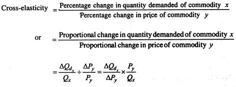
Cross-elasticity varies from minus infinity to plus infinity. Complementary goods have negative cross-elasticities and substitute goods have positive cross-elasticities.

Elasticity of Demand and Supply # 13. Elasticity of Supply:

Much of what we have said about elasticity of demand will hold true for elasticity of supply. Definition of elasticity of supply is very similar.

Elasticity of supply measures the degree of responsiveness of quantity supplied to changes in price.

Thus, the elasticity of supply may be written as:

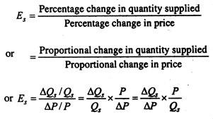
This appears to be identical with the formula for elasticity of demand. However, you will recall that price elasticity of demand is always negative. But price elasticity of supply is normally positive since the supply curve slopes upwards from left to right; except in the case of a backward-bending supply curve, in which case it would have negative elasticity.

Elasticity of Demand and Supply # 14. Classifying Supply Elasticities:

There are three cases of supply elasticity as in Fig. 3.9. SS is a perfectly elastic supply curve, S’S’ is a zero elastic (or perfectly inelastic) supply curve and OS” is a unit-elastic supply curve. Any straight line supply curve that passes through the origin has an elasticity of unity irrespective of steepness of the curve.

Elasticity of Demand and Supply # 15. Price Elasticity of Supply and Length of Time for Adjustment:

We already know that the longer the time allowed for adjustment, the greater the price elasticity of demand. The same proposition also applies to supply.

The longer the time for adjustment, the more price-elastic the supply curve becomes:

1. The longer the time allowed for adjustment, the more firms are able to figure out ways to increase production in an industry.

2. The longer the time allowed, the more resources can flow into an industry through expansion of existing firms.

We, therefore, talk about short-run and long-run price elasticities of supply. The short-run is a time-period during which full adjustment has not yet taken place. The long-run is the time- period during which firms have been able to adjust fully to the change in price.

We can show a whole set of supply curves similar to the ones we did for demand. In Fig. 3.10, when nothing can be done in the short-run, the supply curve is vertical SS, when price is P_e and quantity supplied is Q_e.

With a given price increase to P₁, there will be no change in the short-run in quantity supplied; it will remain at Q_e. Given same time for adjustment, the supply curve will rotate at price P_e to S₁S₁. The new quantity supplied will shift out to Q₁ at P₁. Finally, the long- run supply curve is shown by S₂S₂. The quantity supplied again increases to Q₂ at P₁ and so on.

Elasticity of Demand and Supply # 16. Determinants of Supply Elasticity:

Supply elasticities are very important in economics.

As with demand there are a number of factors which affect elasticity of supply:

(a) Time:

This is the most significant factor as we have seen how elasticity increases with time.

(b) Factor Mobility:

The ease with which factors of production can be moved from one use to another will affect elasticity of supply. The higher the factor mobility, the greater will be the elasticity of supply.

(c) Natural Constraints:

Nature would place restrictions upon supply. If, for example we wish to produce more vintage wine it will take years to mature before it becomes vintage.

(d) Risk-Taking:

The more willing entrepreneurs are to take risks, the greater will be the elasticity of supply. This will be partly influenced by the system of incentives in the economy. If, for example, marginal rate of tax is very high, it may reduce the elasticity of supply.

(e) Costs:

Elasticity of supply depends to a great extent on how costs change as output is varied. If unit costs rise rapidly as output rises, then the stimulus to expand production in response to a price rise will quickly be choked-off by those increases in costs that occur as output increases. In this case, supply will rather be inelastic.

If, on the other hand, unit costs rise only slowly as production increases, a rise in price that raises profits will call forth a large increase in quantity supplied before the rise in costs puts a halt to the expansion in output In this case, supply will tend to be rather elastic.