
In this article we will discuss about the geometrical measurement of price-elasticity of demand.
Case # 1. Value of e in the Case of Curvilinear Demand Curve:
The geometrical measurement of price-elasticity of demand at any particular point on a curvilinear demand curve can be obtained with the help of Fig. 2.5. Suppose that the curve DD in this figure is the curvilinear demand curve for a good and R (p, q) is any point on this curve.
The geometrical measurement of price-elasticity of demand at this point is to be obtained.
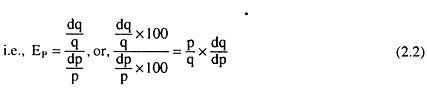
Since dq/dp is the reciprocal of the slope of the demand curve, the formula (2.2) gives us the coefficient of price-elasticity of demand at the point R (p, q) as:
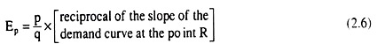
In order to obtain the slope of the demand curve DD at the point R, draw a tangent to the curve at the point R, for the slope of this tangent (AB) itself is the slope of the demand curve DD at the point R—this slope is equal to ![]()
Now putting the values in eq. (2.2), it is obtained:
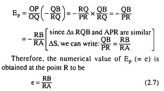
Therefore, to obtain the value of e at any point like R on the curvilinear demand curve DD in Fig. 2.5, draw a tangent to the demand curve at the point R. The value of e is obtained as the ratio of the length of the segment (here RB) of the tangent between R and the horizontal axis and that between R and the vertical axis (here RA).

Case # 2. Value of e at any Point on a Negatively Sloped Straight Line Demand Curve:
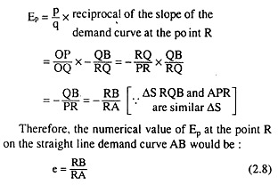
If the demand curve for a good is a negatively sloped straight line like the line AB in Fig. 2.6, then at any point on this line, e.g., at the point R (p, q), the slope of the straight line OA
would be – OA/OB = constant, and Ep at this point would be
ADVERTISEMENTS:
Here e is the ratio of the length of the segment RB of the demand line between the point R and the horizontal axis and that of the segment RA between the point R and the vertical axis.

Case # 3. Negatively Sloped Straight Line Demand Curve: 0 ≤ e ≤ ∞
It can be easily proved that, for a negatively sloped straight line demand curve, the value of e would be different at different prices of the good and e would lie between zero and infinity, both ends inclusive (0 ≤ e ≤ ∞).
Suppose that the negatively sloped straight line AB in Fig. 2.7, is the demand curve for a good. When the price and quantity demanded for the good are OP and OQ, respectively, at the point R on this demand curve. At this point, the value of e is: RB/RA. Now, if the price of the good gets diminishing, the point R would be moving downward towards right along the demand curve AB.
As a consequence of this, the segment RB would be diminishing and the segment RA would be increasing, and so, e = RB/RA would be diminishing. Similarly, if the price of the good increases, the point R would moving upward towards left along the demand curve, and so, the segment RA would be diminishing and the segment RB would be increasing, RB and, therefore, e = RB/RA would be increasing.

ADVERTISEMENTS:
Therefore, it is obtained that as p changes (decreases or increases), e also changes (decreases or increases) along the straight line demand curve. Therefore, along such a demand curve e would be different at different prices.
Now, initially at the point R on the demand curve AB, where p = OP and q = OQ, and, e = RB/RA. If now p diminishes and tends to zero, the point R would approach the point B along the demand curve, the segment RB would be diminishing and it would tend to zero, and the segment RA would be increasing and it would tend to become B A, and therefore, e would tend to be O/BA = 0.
On the other hand, as p increases from OP and tends to become OA, the point R would approach the point A along the demand curve, the segment RA would be diminishing and it would tend to zero, and the segment RB would be increasing and it would tend to become AB, and, therefore, e would tend to AB/0 = ∞.
Therefore, it may now be concluded that if the demand curve for a good is a negatively sloped straight line, then e would be different at different prices and e would lie between zero and infinity, both ends inclusive (0 ≤ e ≤ ∞).
ADVERTISEMENTS:
In the case of such a demand curve (like the line AB) given in Fig. 2.7, shown at what point on this curve e = 1, at what points e > 1 and at what points e < 1. Here, suppose that the midpoint of the line segment AB is R (i.e., RB = RA), and so, it is obtained from simple geometry that OP = OA/2.
Therefore, when the price of the good is OP = OA/2, at point R : e = RB/RA = 1 ( RB = RA). At any point lying on the line AB to the north-west of point R, i.e., at P > OA/2, e > 1 (... RB > RA) and at any point to the south-east of point R, i.e., at P < OA/2, e < 1 (... RB < RA).