Identification Problem of Demand Curve and Supply Curve

In this article we will discuss about the identification problem of demand curve and supply curve.

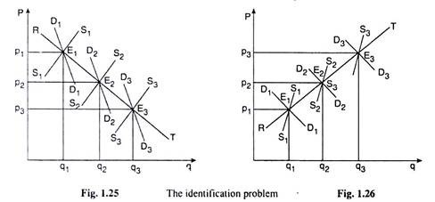
Suppose, for a particular product the equilibrium price-quantity combinations that are observed in the market at different points of time are E₁ (p₁, q₁), E₂ (p₂, q₂), E₃ (p₃, q₃), etc. as shown in Fig. 1.25 or in Fig. 1.26.

From this it may be concluded that, in any of these two diagrams, the quantities demanded (q^d_s) of the product are q₁, q₂ and q₃ at prices p₁, p₂ and p₃, respectively, and so the curve RT joining these points would give us the demand curve for the product.

But it may be very well called RT the supply curve of the product for it also shows that at prices p₁, p₂ and p₃, the quantities supplied (q^s_s) of the product is q₁, q₂ and q₃, respectively. That is, it is confronted with a problem known as the identification problem.

However, if the curve RT has a negative slope like that in Fig. 1.25, it may be inclined to call it the demand curve. On the other hand, if RT has a positive slope like that in Fig. 1.26, it may be inclined to take it as the supply curve.

 

But a look at Fig. 1.25 or Fig. 1.26 would convince us that RT is neither the demand curve nor the supply curve. For Figs. 1.24 and 1.25 give us that the (p, q) combinations at the points E₁, E₂ and E₃ do lie neither on a single demand curve nor on a single supply curve.

Rather, these combinations lie on shifting demand and supply curves at different time-points. For example, in Fig. 1.25, at any particular point of time, E₁ is the equilibrium point being the point of intersection of the demand and supply curves D₁D₁ and S₁S₁.

But, at a different point of time, both these curves have shifted to the right to D₂D₂ and S₂S₂, and now E₂ is their point of intersection. Since both these curves have shifted to the right and the shift in the supply curve has been larger than that of the demand curve, p now has decreased and q increased, giving us the negative slope of the RT curve.

That is, the negative slope of RT is not because it is the demand curve but because of the relative magnitudes of the said shifts in the demand and supply curves.

Similarly, the RT curve in Fig. 1.25 has a positive slope not because it is the supply curve but because both p and q have increased along it owing to shifts in the demand and supply curves.

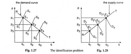
However, if it is assumed, a stable demand curve for the product, which does not shift, i.e., if it is assumed the “other things”, or, the demand determinants other than the price of the good, remain unchanged, then only, the successive shifts in the supply curve may give rise to differ­ent price-quantity combinations at different time-points and, by joining these combinations by a curve, to get the demand curve.

The picture then would look like that in Fig. 1.27. Here, initially, let us suppose, E₁ (p₁, q₁) is the market equilibrium combination at the point of intersection between the (required) demand curve and the supply curve, S₁S₁.

That is, initially, it is obtained q^d to be qi at the price p₁ and E₁ is a point on the demand curve. Now, since the demand curve does not shift, another (p, q) combination at a different time-point may be ob­tained only if the supply of the good changes.

For example, if supply increases and the supply curve shifts to the right, e.g., from S₁S₁ to S₂S₂ in Fig. 1.27, the price of the good would fall from p₁ to p₂ and q^d would rise from q₁ to q₂. This increase in demand would be solely due to the fall in price (because of increase in supply), since the “other things” remain constant.

There­fore, the point E₂ (p₂, q₂) is another point on the demand curve for the good. If the supply curve shifts again to S₃S₃, it get another point E₃ (p₃, q₃) on the demand curve. Therefore, now, as in Fig. 1.27, the curve RT joining the points E₁, E₂, E₃, etc. may be accepted as the demand curve for the good.

Similarly, if it is assumes a stable supply curve which does not shift, i.e., if it is assumed that the determinants of supply other than the price of the good (the “other things” in the case of law of supply) remain unchanged, then only the successive shifts in the demand curve may give rise to different (p, q) combinations at different points of time, and, by joining these combinations by a curve, to get the supply curve of the good. The picture then would look like that in Fig. 1.28.

Here, initially, suppose, E₁ (p₃, q₁) is the market equilibrium combination at the point of intersection between the supply curve and the demand curve, D₁D₁. E₁, therefore, is a point on the supply curve. Now, as the demand curve shifts from D₁D₁ to D₂D₂ to D₃D₃, the equilibrium (p, q) combination moves from E₁ (p₃, q₁ to E₁ (p₂, q₂) to E₃ (p₁, q₃).

Here, since the changes in quantity supplied (q^s) from q₁ to q₂ to q₃ are solely due to changes in price (since the “other things” remain constant), the points E₂ and E₃ are also on the supply curve. Therefore, in Fig. 1.28, the curve RT joining the points E₁, E₂, E₃, etc. would give us the supply curve of the product.

In reality, of course, the demand and the supply determinants other than the price of the good are very unlikely to remain constant over time, i.e., it is almost certain that, in reality, the demand and supply curves would have shifts.

Under the circumstances, to have estimates of demand at various prices on the basis of the time series (p, q) combinations like E₁, E₂, E₃, etc. then it should gather sufficient information about the shift of the demand curve over time.

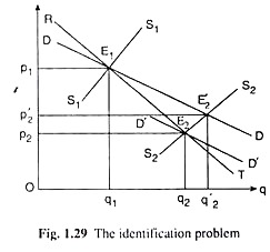
Only then it would be in a position to estimate how much of an increase in demand is due to the shift in the demand curve and how much is due to a fall in the price of the product. It may explain the point with the help of Fig. 1.29.

In Fig. 1.29, suppose that two (p, q) combinations, viz., E₁ (p_b q₁) and E₂ (p₂, q₂) are observed at two different time-points. Of these two combinations, E₁ has been obtained at the point of intersection of the demand curve DD and the supply curve S₁S₁, and E₂ has been obtained at the point of intersection of the demand curve D’D’ and the supply curve S₂S₂.

In this case, since there has been a shift in the demand curve from DD to D’D’, the curve RT joining the points E₁ and E₂ cannot be the demand curve for the good.

However, if it pos­sess sufficient information regarding the shift of the demand curve, it might be possible to ascertain that had there been no shift in the demand curve, then this curve would have been DD, and, in that case, the equilibrium (p, q) combination would have been E’₂ (p₂,q₂) at the point of intersection of the DD and S₂S₂ curves.

Therefore, here the demand curve for the good would be actually DD passing through the points E₁ and E₂ and not RT which is obtained by joining E₁ and E₂. It is identified the actual supply curve of the good from among the shifting supply curves in a similar way, if it possess sufficient information about the shift in the supply curve.