The Negative Sloping of Demand Curve (With Diagram)

The following points highlight the two main approaches that explains the Negative Sloping of Demand Curve. The Approaches are: 1. Cardinal Approach to Demand Analysis 2. Ordinal Approach Indifferent Curve.

Approach # 1. Cardinal Approach to Demand Analysis:

A utility function may be defined as the descriptive statement that relates satisfaction to the consumption of (private) good and services.

It can be written as:

Utility = f (goods, services)

By utility we mean want-satisfying power of a commodity. Such power exists in material things. Anyway, a commodity is demanded because it has utility. Negative sloping demand curve is often explained in terms of utility analysis.

According to Marshall, utility derived from a commodity can be measured in cardinal numbers, like 1, 2, 3, etc., just as we can measure the temperature of human body. Marshall intended to measure utility by an imaginary unit called ‘util’.

Utility is an abstract concept and its units are arbitrary. Further, he suggested the measurement of utility obtained from a commodity in terms of money. When a consumer spends Rs. 5 to buy a kilogram of potato it means his utility equals 5. Hence the name cardinal measurement of utility.

Law of Diminishing Marginal Utility:

Before explaining this celebrated law in economics, we must know the meanings of total utility and marginal utility:

(i) Total Utility (TU):

Total utility refers to the total satisfaction or total benefit derived from the entire consumption of a commodity. Normally, greater the volume of consumption, greater is the level of total satisfaction. This means that the total utility function reflects the quantitative relationship between the satisfaction yielded by a private good and its rate of consumption.

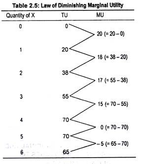
We are assuming that utility is measured in terms of util. Table 2.5 shows the volume of TU obtained by an individual from the consumption of good X. Table 2.5 tells us that as the consumer consumes more and more of X, his TU rises.

For the first unit of X he gets utility of 20 utils, for the second 38 utils, and so on. However, when the consumer consumes the fifth unit, his TU remains unchanged at 70 utils. Consumption of the sixth unit causes a decline in TU.

(ii) Marginal utility (MU):

Marginal utility means change in TU following a change in the consumption of the commodity, i.e.,

MU = change in total utility/change in the quantity of a good

MU, thus, is an addition to or subtraction from TU. In other words, MU is the difference in TU arising from a change in the use of the last unit of the commodity. Table 2.5 states that an individual gets utility of 55 utils from the third unit and 70 utils from the fourth unit.

So his MU becomes 15 utils. Thus, MU for the fourth unit is the difference in TU from the fourth and the third unit of X. Or MU for the nth unit of a good is the difference between TU of nth unit and n – 1th unit i.e., the previous unit:

MU_n = TU_n – TU_n-1

(iii) Law of Diminishing MU:

One of the fundamental laws relating to the tastes and preferences of the consumer is the law of diminishing MU, and not TU. Whenever a particular commodity is consumed its desiredness, i.e., marginal utility to a consumer, on an average, tends to decline. This is the essence of this law that corresponds to our common sense notion or in Marshall’s words: “familiar and fundamental tendency of human nature.”

The law can be stated in the following way:

Other things remaining the same (i.e., money income, tastes and preferences, prices of goods, etc., remaining unchanged), the more one consumes a commodity, his MU will eventually decline.

Or more and more consumption of a commodity will cause MU to decline ultimately. The rate of decline may not be uniform for all commodities. What is true is that the tendency of diminishing MU will ultimately arrive.

This law can be stated in Marshall’s own words:

”The additional benefit which a person derives from a given increase of a stock of a thing diminishes with every increase in the stock that he already has.”

Table 2.5 suggests that as consumption of X rises, TU also rises. Our consumer gets more and more satisfaction as he consumes more of X; but his MU gradually declines. When TU is maximum, MU becomes zero (i.e., for the fifth unit of X).

This means extra consumption of good X adds less and less to his TU. In other words, the rate of increase in TU declines. If the consumer decides to consume the sixth unit of good X, his TU will fall and MU will become negative. In other words, our consumer, in this situation, gets dissatisfaction or disutility. This tendency of a commodity is known as the ‘law of diminishing marginal utility’.

The law of diminishing marginal utility says something about “all you can eat” special. It is quite likely that an individual will stop eating once MU from eating food is zero. At this point total utility is maximum. Consumption beyond this will cause TU to decline and distaste for food will grow in the minds of the consumer.

The relationship between TU and MU can be summarized in the following form:

If TU:

(a) Increases at a diminishing rate

(b) Is maximum

(c) Declines

Then MU:

(a) Declines

(b) Is zero

(c) Becomes negative.

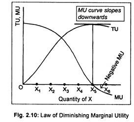
This law can be illustrated with the help of a diagram. In Fig. 2.10 we measure quantities of X consumed on the horizontal axis and both TU and MU of X on the vertical axis.

The figure suggests that the TU curve gradually rises, reaches a peak, and from there it declines. On the other hand, MU curve gradually declines. When OX₅ units of X are consumed, TU becomes maximum and MU becomes zero. To understand this, we have drawn a tangent at the highest point of the TU curve. As the tangent is parallel to the horizontal axis, TU is maximum there.

Remember that the slope of TU curve is the MU. The slope of TU at its maximum point is zero. So MU must be zero. If a consumer consumes OX₆ units of good X, TU will decline and MU will be negative. Here the MU curve cuts the horizontal axis indicating disutility. Anyway, the tendency of the MU curve to slope downwards from left to the right is suggestive of the law of diminishing MU.

(iv) Assumptions behind the Law:

The Marshallian law of diminishing MU will come into operation provided certain assumptions are made:

a. Utility derived from a commodity is cardinally measurable.

b. Marginal utility derived from a commodity tends to diminish.

c. Marginal utility of money remains constant.

d. Money income, tastes and preferences, prices of substitute and complementary goods etc., remain unchanged.

(v) Exceptions:

Obviously, if any of the assumptions do not hold, the law may not be operative.

Exceptions to this Law are:

Firstly, utility, being a psychological concept, cannot be measured in cardinal numbers. It varies from person to person and from place to place.

Secondly, like commodities, MU of money may also diminish. It does not remain invariant to a consumer when his stock of money changes. More and more purchase of commodities means fall in the stock of money. In such a situation, MU of money should rise. When stock of money rises, MU of money should decline.

Thirdly, the law may not be applicable in the case of articles of hobby. Usually, a postal stamp collector has an unending appetite for additional stamps. Naturally, the law of diminishing MU for this commodity does not hold.

Fourthly, the law of diminishing MU may not hold if a consumer gets very little quantity of a commodity. For a thirsty man, drops of water consumed in several doses may not exhibit the law of diminishing MU.

Despite these limitations, the law usually holds. In other words, the above-noted exceptions are not true exceptions to this law. The law can be postponed for the time being but the law is more likely to appear eventually. The law appears to be an empirical one. That is why this law explains the law of demand.

Derivation of Demand Curve from the Marginal Utility Curve:

By equilibrium, we mean a state of balance or rest. The basic objective of a consumer is the maximization of satisfaction from the consumption of goods. A consumer reaches equilibrium when he gets maximum satis­faction or maximum total utility. After getting maximum utility a consumer does not find any interest in changing his consumption pattern. He, thus, comes to a rest.

The concept of marginal utility is employed to explain the equilibrium of a consumer. The marginal utility curve is also employed to derive the demand curve for a commodity.

Before describing the equilibrium of a consumer in a single commodity framework, we must assume:

a. Utility is cardinally measurable.

b. Marginal utility of a commodity diminishes but marginal utility of money remains constant.

c. Price of the commodity, money income etc., do not change.

d. Our representative consumer acts rationally in the sense that he is neither an extravagant nor a miser.

The tastes and preferences of the consumer are represented by the marginal utility (MU) curve which is indeed negative sloping. Given the limited money income and the product price, the rational consumer sets out to maximize his ‘net’ utility.

Net utility is the difference between marginal utility obtained from a commodity and the price sacrificed to have this commodity. His net utility becomes maximum when marginal utility (measured in money units) equals the price of the product. Thus the condition for equilibrium of a consumer for good X is reached when MU_X = P_X.

A consumer spends his given money income in such a way that the marginal utility of the last unit purchased is equal to the price of the product. If MU_X ≠ P_X, the consumer will go on either consuming more or less until equality is restored.

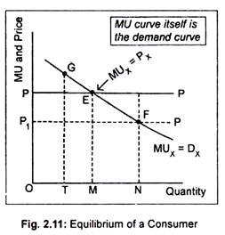
Clearly, a consumer can increase his total utility by purchasing more or less as long as the value he places on each additional unit exceeds or falls short of the amount he must pay. In Fig. 2.11, we have drawn MU curve for good X which exhibits the law of diminishing MU.

We measure quantities of good X on the horizontal axis and price as well as MU obtained from X on the vertical axis. To explain constancy in price, we have drawn PP line as parallel to the horizontal axis. At this given price, the consumer is at liberty to buy any amount he likes.

As long as MU_X exceeds P_X, it is profitable to purchase more of X. Suppose, our consumer buys OT of X. Since MU_X > P_X, the consumer can increase his utility by purchasing more of X. It will continue until point E is reached where MU_X = P_X. At this point, the consumer reaches equilibrium and gets maximum satisfaction by buying OM units of good X.

Similarly, when the consumer purchases ON of good X, his sacrifice is larger than the utility obtained, i.e., P_X > MU_X. So, a consumer will reduce his purchases in order to maximize net utility until point E is reached. Thus, E is the equilibrium point where our consumer gets highest satisfaction.

Derivation of a Demand Curve:

Now we will derive a demand curve showing price-quantity relationship. When the consumer consumes one commodity, the marginal utility schedule itself for this commodity becomes the demand curve.

We know that a consumer—with his limited money income and given price of the product—will go on purchasing a commodity to obtain the greatest satisfaction until marginal utility for the commodity is equal to its price. This is shown in Fig. 2.11 where E is the initial equilibrium point. Now by varying the price, we can derive another set of equilibrium points to obtain a demand curve.

In Fig. 2.11, our consumer demands OM of good X when its price is OP. Note that corresponding to this amount of consumption, MU_X = P_X. If price of X falls to OP₁, a new equilibrium point F is obtained. Corres­ponding to point F, the consumer purchases a larger quantity of X, i.e., ON. This means that, at a lower price, a larger quantity is demanded.

Thus, the MU_X curve itself is the demand curve for X which is inclined negatively throughout the length. So, we can conclude that the demand curve for a normal good is negatively sloped due to the operation of the law of diminishing marginal utility.

Approach # 2. Ordinal Approach: Indifference Curve:

Modern economists like Hicks and Allen have rejected the cardinal measurement of utility. On the other hand, their approach is known as ordinal approach. A consumer can rank his preference out of various commodity bundles. That is to say, utility—though not measurable —is comparable.

If a consumer is presented with a number of various combinations (say, A, B, C) of two goods, he can rank them in a scale of preferences. A consumer can say that A is preferable to B or B to A. But he can’t say that from A he gets maximum satisfaction of 10 units.

Assumptions:

Before defining indifference curve, we must make the following assump­tions:

(i) Completeness,

(ii) Non-satiety; and

(iii) Consistency and transitivity.

(i) Completeness:

For simplicity’s sake, let us assume that there are two goods, X and Y, containing various quantities of these two goods.

We also assume that preferences are complete. This means that a consumer can determine which combination of X and Y is preferable or which combinations of X and Y yield the same level of satisfaction. Since the consumer knows the ‘utility value of all possible choices’ economists say that preferences are complete.

(ii) Non-Satiety:

The assumption of non- satiety states that a consumer always prefers ‘more of a commodity to less’. Let situation A contain more of good X and good Y than the situation B. Obviously, A would be preferred to B since more is preferred to less.

(iii) Consistency and Transitivity:

The consumer is also expected to behave consistently. If a consumer prefers A to B in any situation then he must not choose B over A in the other situation. If, however, he chooses B, then his behaviour is said to be contradictory and inconsistent.

Further, preferences must be transitive. This means that if a consumer chooses A over B and B over C then he chooses A over C. If that were not true, then consumer preferences would not be transitive. Thus the assumption of consistency is related to the assumption of transitivity.

These three assumptions enable us to represent consumer preferences in a graphic form. As a result, we obtain the indifference curve.

(a) Meaning of Indifference Curve:

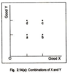
In Fig. 2.14(a), we measure good X on the horizontal axis and good Y on the vertical axis, a, b, c and d are the four combinations of X and Y. All these combinations may be either-preferred by the consumer or a consumer may be indifferent among these combinations.

Rationality or non-satiety assumption states that more is always preferred to less. Thus, c is preferred to a, b or d, since c contains larger combinations of X and Y. Likewise, d is preferred to a. But we are not sure whether d is preferred to b or b is preferred to d.

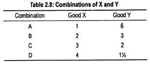
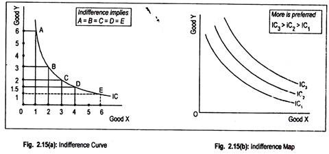
If no preference is observed between d and b, we can assume that the consumer is indifferent between combinations d and b. Connecting these two points, we obtain the indifference curve shown in Fig. 2.15(a). Before describing this figure, we use Table 2.8 to derive an indifference curve.

Suppose a consumer purchases various combinations of goods X and Y as shown in Table 2.8. Our consumer gets the same level of satisfaction from X and Y whether he purchases combination A or B or C or D. To him, all such combinations give the same level of satisfaction. That is why he is indifferent between different combinations.

This table can be represented with the help of Fig. 2.15(a) where we measure goods X and Y on the horizontal and vertical axes, respectively. Point A on the curve IC denotes 1 unit of X and 6 units of Y. Point B denotes 2 units of X and 3 units of Y. Similarly, points C and D denote the use of more X and less Y. By joining these points we get a curve known as indifference curve, IC.

Our consumer is indifferent between all these points. He can’t say which point is giving him the maximum satisfaction.

All the points give him the same level of satisfaction. Thus, an indifference curve represents various combinations of goods X and Y that yield the same amount of satisfaction to the consumer. As he cannot say which combination of the two goods gives him the highest satisfaction, he is, therefore, indifferent between the combinations. Hence the name indifference curve.

Indifference Map:

A set of indifference curve plotted on a graph is called an indifference map. A consumer is indifferent on an indifference curve and not between two indifference curves. Higher (lower) indifference curve represents higher (lower) level of satisfaction.

A consumer can have more of both the goods if he experiences, say, an increase in income. In Fig. 2.15(b), an indifference map has been drawn. IC₁ is the lower order indifference curve. IC₂ is the higher order indifference curve that contains more of both X and Y. Thus, IC₂ is preferable to IC₁. That is to say, IC₃ > IC₂ > IC₁. An indifference map consists of more than one indifference curves.

In other words, an indifference map is a family of indifference curves.

Characteristics of Indifference Curve:

An indifference curve has three important properties:

(i) An Indifference Curve Must Slope Downwards from Left to the Right:

Proof:

It is clear from Fig. 2.15(a) that if the consumer travels from point A to B, he tends to consume more of X and less of Y. Similarly, the consumer purchases more of X and less of Y if he moves from point B to C or from C to D. This must be so if the level of satisfaction is to remain the same on an indifference curve. Thus an indifference curve must have a negative slope.

Proof of this negatively sloped indifference curve can also be made with the help of Fig. 2.16. In Fig. 2.16(a), IC is drawn parallel to the vertical axis indicating that as a consumer moves from A to B to C, his consumption of Y rises while that of X remains the same.

The consumer is indifferent between having more or less of the good X. Thus, X is a ‘neuter’ good. This flat indifference curve implies that if we take 1 unit of good X away at point A, then we need not compensate the consumer for this loss of good X with any amount of Y to keep him on the same indifference curve.

In Fig. 2.16(b), as IC is parallel to the horizontal axis, consumption of X rises and that of Y remains unchanged. By the same logic, good Y is a ‘neuter good’. To have a negatively sloped indifference curve, consumption of one good must increase while that of another must decline. Indifference curve can never be upward rising as shown in Fig. 2.16(c).

As a consumer moves from A to B to C, his consumption of both X and Y rise. This shape of indifference curve is also ruled out as non- satiety assumption—i.e., more is preferred to less— will be violated. Thus, an indifference curve must be downward sloping.

(ii) An Indifference Curve is Convex to the Origin. Or it is Concave from above:

Proof:

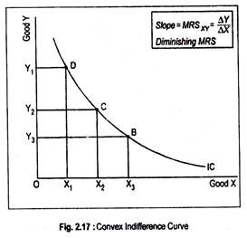
An indifference curve is convex to the origin because of diminishing marginal rate of substitution between two goods, X and Y. Marginal rate of substitution of X for Y (MRS_XY) represents the amount of Y which the consumer gives up for an additional unit of X so that his satisfaction remains intact. As the rate of substitution diminishes the curve must be convex to the origin. This has been explained with the help of Fig. 2.17.

If a consumer moves from D to C, he sacrifices Y and takes up more X. It means that the loss of satisfaction caused by giving up Y₁Y₂ of Y equals the gain in satisfaction due to the increase in good X by X₁X₂.

Thus, the marginal rate of substitution is:

OY₁ – OY₂/OX₂ – OX₁= DE/EC

Similarly, if he moves from C to B, the marginal rate of substitution becomes:

OY₂ – OY₃/OX₃ – OX₂ = CF/FB

However, DE/EC > CF/FB.This means that initially the consumer was prepared to sacrifice more of Y for X. But, as he slided down the curve, his stock of Y diminishes and stock of X increases. This suggests that he is willing to give up less and less of Y for a given increment in X. Thus, the marginal rate of substitution of X for Y falls as the consumer possesses more of X and less of Y. So, an indifference curve must be convex to the origin.

It is to be remembered that the slope of an indifference curve is MRS. The slope is -∆Y/∆X. Thus, the slope of an indifference curve is negative.

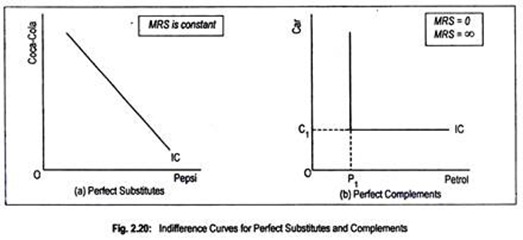
Anyway, if the indifference curve is steep (flat) MRS will be high (low). If two goods are perfect substitutes, then indifference curve would be a straight line and MRS would be constant (Fig. 2.20a). For complementary goods, indifference curve becomes L-shaped (Fig. 2.20b).

On the other hand, an indifference curve can never be concave to the origin since the marginal rate of substitution becomes increasing.

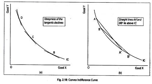
Slope at a point on an indifference curve can be measured by drawing a tangent to that particular point. At points D, C and B on an indifference curve, we have drawn three tangents in Fig 2.18(a). As we move downwards, steepness of the tangent declines. Slope of the tangent at D is steeper than the tangent at C or B. This means that the slope or MRS declines.

So, an indifference curve must be convex to the origin. Or simply, if an indifference curve lies above a tangent line drawn at any point on the curve, the curve is said to be convex to the origin (Fig. 2.18(a)).

Again, if a straight line connecting any two points (say AA’ or BB’) on the curve lies above the curve IC (Fig. 2.18(b)), the curve is convex to the origin.

On the other hand, if the tangents lie above the curve, and a chord connecting two points on the curve lies below the curve, the indifference curve becomes concave to the origin.

(iii) No Two Indifference Curves Can Touch or Intersect Each Other:

Proof:

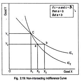
If two curves intersect or touch each other we will get an absurd result. This is shown in Fig. 2.18 where IC₁ and IC₂ have cut each other at point c. Points a and c lie on IC₂ and points- b and c lie on IC₁. As points a and c lie on IC₂, these two points must represent the same level of satisfaction, that is,

OX₁ + OY₁ = 0X₂ + OY₂ … (2.1)

Similarly, from point’s c and b on IC₁, we get

OX₁ + OY₁ = OX₃ + OY₂ … (2.2)

As the L.H.S. of (2.1) and (2.2) are the same, it follows, therefore

OX₂ + OY₂ = OX₃ + OY₂

Or OX₂= OX₃

But, it is clear from the figure that OX₃ > OX₂. Transitivity assumption is thus violated. So, two indifference curves must not cut each other.

Indifference Curve for:

(i) Perfect Substitutes, and

(ii) Perfect Complements

Goods are substitutes that compete in the market, so that if the price of one good increases, the quantity demanded for another will also increase. Two goods are perfect substitutes if the quantity demanded of one good is positively related to the price of the other. Pepsi and Coca-Cola cold drinks, tea and coffee, etc., are perfect substitutes.

For such substitutes, indifference curve becomes a negative sloping straight line since a consumer is entirely indifferent between having a Pepsi bottle or the Coca-Cola bottle. For substitute goods, MRS_XY is constant and has always a slope of (—) 1. A consumer thus gives up the same number of Pepsi for another Coca-Cola, or vice versa. At a constant rate, substitution takes place.

Goods that are used jointly with each other are called complements. Petrol and car, right shoe and left shoe are complements. As these are complements to each other, a fall in the price of either will increase the demand for both. In this case, an indifference curve becomes L-shaped.

Here both the goods are consumed in fixed proportions:

Always OP₁ units of petrol and OC₁ units of car will be used. One cannot have more of petrol and less of car or more of car and less of petrol. Thus, MRS becomes either zero or infinity and nothing in-between.

Some Unusual Shapes of Indifference Curve:

We have drawn negatively sloped indifference curve for two goods X and Y. These goods are treated as ‘good’ as they are deemed to be fit for consumption. In other words, when goods are ‘good’, indifference curve is negative sloping and convex to the origin.

But, sometimes, to a consumer some of the goods may become ‘bad’ or unfit for consumption. This means that a consumer gets less satisfaction by consuming more of that (‘bad’) commodity. Thus, the ‘good’ becomes a ‘bad’. In this case, the consumer will get more satisfaction if he consumes less and less of the ‘bad’ commodity. An example of such ‘bad’ good is pollution.

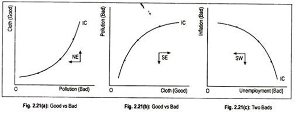
‘Bad’ good is measured on the horizontal axis, while a ‘good’ commodity is measured on the vertical axis in Fig. 2.21(a). Now the indifference curve is upward sloping. A consumer would get higher satisfaction if he consumes less of the ‘bad’ good.

If the consumer consumes more of a ‘bad’ good then the consumer needs more of the ‘good’ good to stay on the same indifference curve. In Fig. 2.21(b), an indifference curve is also upward sloping for ‘good’ and ‘bad’ goods.

If the two goods are ‘bads’ (say, unemploy­ment and inflation) then indifference curve would look like Fig. 2.21(c). Here the indifference curve looks like indifference curves for two ‘good’ goods, but it has the opposite curvature. In this case, an indifference curve is concave to the origin.

Let us now suppose that a particular good is a ‘neuter’ or ‘neutral’ good in the sense that the consumer does not bother whether he consumes more or less of that commodity. However, the other commodity may be ‘normal’ or ‘good‘. In such a situation of normal and neuter good, indifference curve would look like either Fig. 2.16(a) or 2.16(b), (P. 46).

If good X is a neuter one while good Y is a normal one then the indifference curve would be parallel to the vertical axis. Indifference curve would be parallel to the horizontal axis if good X (neuter good) is measured on the horizontal axis.

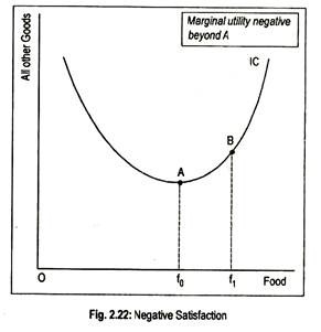
There are some commodities which provide a negative satisfaction if they are consumed beyond a certain level even if they are ‘free’ good. If one of the two goods is of this type, then indifference curve would be positive sloping. It is because the consumer is willing to sacrifice some amount of the other good to be permitted to reduce his consumption of the ‘offending’ commodity.

This is shown in Fig. 2.22 where Of₀ amount of a commodity, say food, is consumed. At point A, the slope of the indifference curve becomes zero and, hence, MRS is zero. As consumption of food beyond Of₀ yields negative utility, the indifference curve becomes positive sloping.

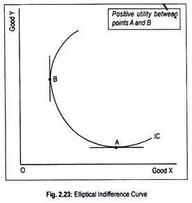
In Fig. 2.23, another unusual shaped indifference curve has been drawn. At point A on this curve marginal utility of X is zero and, at point B, marginal utility of Y is zero. Consumption beyond point A implies negative utility for X and consumption beyond point B yields negative utility for Y. Between points A and B, marginal utilities for both X and Y are positive.