3 Main Types of Cost Functions

The following points highlight the three main types of cost functions. The types are: 1. Linear Cost Function 2. Quadratic Cost Function 3. Cubic Cost Function.

Type # 1. Linear Cost Function:

A linear cost function may be expressed as fol­lows:

TC = k + ƒ (Q)

where TC is total cost, k is total fixed cost and which is a constant and ƒ(Q) is variable cost which is a function of output.

It may alternatively be expressed as:

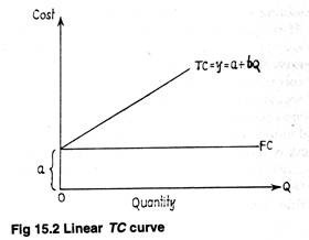
TC = Y = a + bQ.

It is depicted in Fig. 15.2. The cost function here is derived from the basis of following (implicit) assumptions:

(i) When output is zero, total cost is equal to total fixed cost. Moreover, the shorter the short run, the more certain is the manager that fixed costs are sunk (historical) costs by definition. If total fixed cost remains constant at all levels of output up to capacity, any increase in total cost is traceable to change in total variable cost.

To be more specific, if factor prices remain constant over the relevant range of output, a doubling of inputs would lead to an exactly doubling of output. In other words, there would be constant returns to the variable factor.

(ii) We assume away the operation of the Law of Diminishing Returns. The linear cost function in Fig. 15.2 reflects the short run cost condition of the firm. In the short run, capacity (or plant size) is fixed. So the firm can vary its level of rate of output up to capacity (i.e., with the existing plant).

(iii) Average (total) cost declines with an expan­sion of output.

Average cost may be expressed as:

AC = Y/Q

where Y is total cost and Q is output.

Marginal cost may be expressed as:

MC ∆Y/∆Q = b

If-the cost function is continuous, marginal cost may be expressed as

MC = d (TC)/ dQ

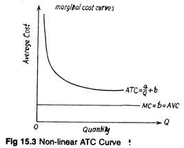
In both the situations, MC = b and MC is con­stant and is a linear cost equation. Such a constant MC curve appears as horizontal line parallel to the output axis as in Fig. 15.3.

The shorter the short run the greater the likeli­hood that statistical cost functions will have a bias towards linearity. This bias may, as Coyne argues, “may be justifiable and, in fact, reasonably valid if it occurs over the relevant range of a firm’s TPP curve. Extrapolation of linear cost functions requir­ing output beyond the relevant range in either direc­tion and used for predictive purposes will generate misleading and statistically insignificant results.”

If we apply the linear cost function in the cricket bat example we observe that the cost curve assumes the existence of a linear production function. If a lin­ear cost function is found to exist, output of cricket bat would expand indefinitely and there would be a one-to-one correspondence (relationship) between total output and total cost.

In other words, dimin­ishing returns to the variable factor would not be observed. Such a function would exist for the cricket bat factory only if the relevant range of output under consideration was very small.

Type # 2. Quadratic Cost Function:

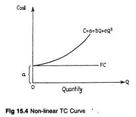
If there is diminishing return to the variable fac­tor the cost function becomes quadratic. There is a point beyond which TPP is not proportionate. Therefore, the marginal physical product of the vari­able factor will diminish.

And if TPP actually falls MPP will be negative. In other words, there is a point beyond which additional increases in output cannot be made. So costs rise beyond this point, but output cannot. Such cost function is illustrated in Fig. 15.4.

We have noted that if the cost function is linear, the equation used in preparing the total cost curve in Fig. 15.2 is sufficient. But the quadratic cost func­tion has one bend – one bend less than the highest exponent of Q.

Total cost is equal to fixed cost when Q — 0, i.e., when no output is being produced. However, as Q increases, fixed cost remains unchanged. Therefore, increases in total costs are traceable to changes in variable cost.

It is to be highlighted that the major difference between the linear and quadratic cost functions is the area of diminishing returns to the variable fac­tors). If the cost function is linear, variable cost increases at a constant rate.

It is quite reasonable to assume that linear cost functions exist regardless of the current level of operating capacity at which the firm is producing. Rather, the truth is that as output reaches the physical capacity limitations of existing plant and equipment in the short run, vari­able costs rise because of the operation of the Law of Diminishing Returns (or variable proportions).

Most economists agree that linear cost functions are valid over the relevant range of output for the firm. Over this range of output, “no statistically significant improvement on the linear hypothesis is achieved by the inclusion of second or higher degree terms in output”; moreover, “supplementary tests, such as the examination of incremental cost ratios, , usually confirm the linear hypothesis.”

Type # 3. Cubic Cost Function:

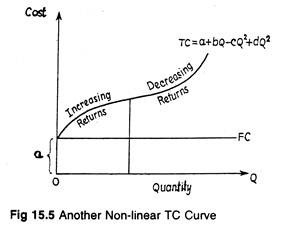
In traditional economics, we must make use of the cubic cost function as illustrated in Fig. 15.5. Such a cost function is not of much empirical use. It does not provide statistically significant improve­ments over the linear or quadratic cost function. Moreover, it is very difficult to calculate, interpret and apply, to test statistical hypothesis regarding cost behaviour in manufacturing concerns.

The cubic cost function is based on three im­plicit assumptions:

1. When Q = 0, total cost is equal to total fixed cost.

2. Total fixed cost remains constant at levels of output up to capacity (as in the previous two cases).

3. With an output expansion there is an ini­tial stage of increasing return to the variable factor; thereafter a point is reached (the inflection point) at which there is constant return to the variable factor; finally, there is diminishing return to the variable factor. In short, the cubic cost curve has two bends, one bend less than the highest exponent of Q.