The following article will guide you about how are a firm’s short run average and marginal cost curves derived.
Just as the average and marginal product curves were derived geometrically from the total product curve, the average and marginal cost curves may also be derived from the corresponding total cost curve.
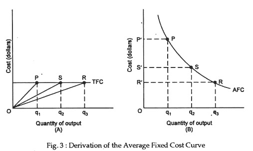
Figure 3 illustrates the derivation of average fixed cost.
(Note: Vertical axes of panels A and B have different scales.) In panel A, total fixed cost is plotted and the outputs Oq1, Oq2 and Oq3 are measured so that Oq1 = q1q2 = q2q3.
Since AFC = TFC/Q, average fixed cost is given by the slope of a ray from the origin to a point on the TFC curve. For output Oq1, AFC is the slope of the ray OP, or q1 P/Oq1. Similarly, for output Oq2, AFC is q2S/Oq2, and so on. Since TFC is always the same, q1P = q2S = q3R. By construction, Oq2 = 2Oq1 and Oq3 = 3Oq1.
Thus AFC for output Oq2 is q2S/Oq2 = q1P/20q1 = 1/2 (q1P/Oq1) = 1/2 AFC for output Oq1. This is shown in panel B by the difference in OP’ and OS’ — more specifically, OS’ = 1/2 OS’. Similarly, as you can demonstrate for yourself, OS’ =1/3 OF. The remaining points on AFC are determined in the same way.
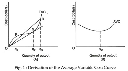
Figure 4 shows how AVC is derived from TVC. As is true of all “average” curves, the average variable cost associated with any level of output is given by the slope of a ray from the origin to the corresponding point on the TVC curve. As may easily be seen from panel A, the slope of a ray from the origin to the curve steadily diminishes as one passes through points such as P; and it diminishes until the ray is just tangent to the TVC curve at point S, associated with output Oq2.
Thereafter the slope increases as one moves from S toward points such as R. This is reflected in panel B by constructing AVC with a negative slope until output Oq2 is attained. After that point, the slope becomes positive and remains positive thereafter.
ADVERTISEMENTS:
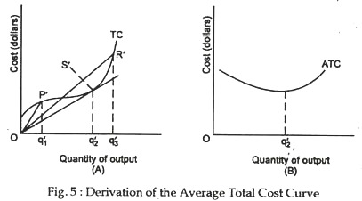
Exactly the same argument holds for panels A and B of Figure 5 which show the derivation of ATC from TC. The slope of the ray diminishes as one moves along TC until the point S’ is reached. At S’ the slope of the ray is least, so minimum ATC is attained at the output level Oq2. Thereafter, the slope of the ray increases continuously, and the ATC curve has a positive slope.
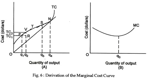
Finally, the derivation of marginal cost is illustrated in Figure 6. Panel A contains the total cost curve TC. As output increases from Oq1 to Oq2, one moves from point P to point V, and total cost increases from TC1 to TC2.
Now let the point P move along TC toward point V. As the distance between P and V becomes smaller and smaller, the slope of the tangent T at point V becomes a progressively better estimate of VR/PR. And in the limit, movements in a tiny neighborhood around point V the slope of the tangent is marginal cost.
As one moves along TC through points such as P and V, the slope TC diminishes. The slope continues to diminish until point S is reached output Oq3. Thereafter the slope increases. Therefore, the MC curve is constructed in panel B so that it decreases until output Oq3 is attained increases thereafter.
One final point should be noted about Figures 5 and 6. TC and TVC have the same slope at each output point: TC is similarly TVC displaced upward by the constant amount TFC. Since the slopes is the same, MC is given by the slope of either curve.
In panel A, Figure 5, the slope of the ray OS gives minimum AFC. But at this point the ray OS is just tangent to TVC; hence it also gives MC at this point. Thus MC = ATC when the latter attains its minimum value. Similarly, in point A, Figure 6, the slope of the ray ON gives minimum ATC. But at the point the ray is tangent to TC; thus its slope also gives MC. Consequently MC = ATC when the latter attains its minimum value.
Short-Run Cost Curves:
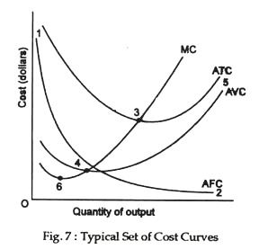
The properties of the average and marginal cost curves are illustrated by the “typical” set of short-run cost curves shown in Figure 5.
The properties may be summarised as follows:
Relations:
(i) AFC declines continuously, approaching both axes asymptotically as shown by points 1 and 2 in the Fig. 7. AFC is a rectangular hyperbola,
(ii) AVC first declines, reaches a minimum at point 4, and rises thereafter. When AVC attains its minimum at point 4, MC equals AVC. As AFC approaches asymptotically close to the horizontal axis, A VC approaches ATC asymptotically, as shown by point 5,
(iii) ATC first declines, reaches a minimum at point 3, and rises thereafter. When ATC attains its minimum at point 6, and rises thereafter MC equals ATC,
(iv) MC first declines, ATC when these curves attain their minimum values. Furthermore, MC lies below both AVC and ATC over the range in which the curves decline; it lies above them when they are rising.
