In general, the learning curve relationship is expressed as a constant percentage. This percentage represents the proportion by which the amount of an input (or cost) per unit of output is reduced each time production is doubled. For instance, consider a production process in which labour input and costs follow an 80% learning curve.
Assume that the first unit requires labour costs of $1, 000 to produce. So the second unit will cost $1,000 x .80 = $800, the fourth unit $640(= $800 x .80), the eighth unit $512(= $640 x .80), the sixteenth unit $409.60(= $512 x .80), and so on.
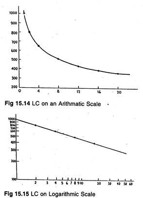
The learning curve relationship may also be shown diagrammatically. See Fig. 15.14 and 15.15. In Fig. 15.14 it is plotted on an arithmetic scale and the cost output relationship is a curvilinear function. In Fig. 15.15, it is plotted on a logarithmic scale and the cost-output relationship is a linear function.
The learning curve relationship is usually expressed as:
ADVERTISEMENTS:
C = aQb (1)
where C is the input cost of the Qth unit of output, Q is consecutive units of output produced, a is the theoretical (or actual) input cost of the first unit of output, and b is the rate of decline in input cost per unit of output. The value of 6 is normally negative because the learning curve is downward sloping.
Equation (1) can be converted into linear form by taking logarithms:
ADVERTISEMENTS:
log C = log a + b log Q (2)
In logarithmic form, b represents the slope of the function.
Estimating the Learning Curve Parameters:
The learning curve is often applied for cost and profit forecasting. For this, one has to first determine the values of the log a and b parameters in equation (2). If we do not have any historical cost output data for the production process, we should make subjective estimates of these parameters based on prior experience with similar type of production operations.
ADVERTISEMENTS:
However, for an established production process, historical cost-output data are available. In this case, the least-squares technique of regression analysis can be applied to estimate the parameters.
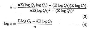
In equation (2), log C is the dependent variable and log Q is the independent variable. If we apply the least-squares procedures to the series of cost-output observations we derive the following equations for estimating the learning curve parameters.
where n is the number of observations.
Example 1:
The Chloride Ltd., manufacturer of Exide batteries, is trying to develop a learning curve model to help forecast labour costs for successive units of one of its products. From the past data, the company knows that the labour costs of the 25th, 75th and 125th units were Rs. 800, Rs. 600 and Rs. 500, respectively.
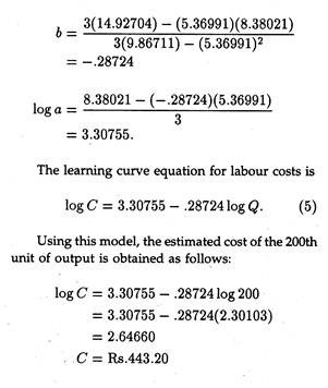
Develop the learning curve equation from this data and use the resulting model to predict labour costs for the 200th unit of output. The preliminary calculations needed to determine logo and 6 are shown in Table 15.2. Substituting the column totals from the last row of Table 15.2 into equations (3) and (4) provides the following estimates of the learning curve parameters:
The Percentage of Learning:
The percentage of learning which is defined as the proportion by which an input (or its associated cost) is reduced when output is doubled, can be estimated as follows:
ADVERTISEMENTS:
L =C2/C1 100% (6)
where C1 is the input (or cost) of Q1 units of output, and C2 is the cost for the Q2= 2Q1 units of output. In order to illustrate the calculation of the percentage of learning, revert to the Chloride example again. Using the learning curve model developed earlier (equation 5), labour costs for Q1 — 50th units of output are C1= Rs. 659.98 and labour costs for 2Q1 = 100th units of output are C2= Rs. 540.84.
Substituting these values into equation (6) yields:
ADVERTISEMENTS:
L = 540.84/659.98 x 100% = 81.9%
The percentage of learning for labour costs in the production of these battery units is thus, approximately, 82%. This implies that labour costs decline by about 18% each time output is doubled.
Effects of Learning Curves on Variable Costs per Unit and Profit:
A common form of learning curve is based on reduction of labour hours per extra unit of output by a constant fraction each time the total output is doubled.
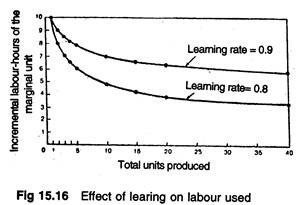
Suppose the labour requirement is reduced by 10% with each doubling of output. Incremental labour requirement for the ith unit is 0.9 times the incremental labour needed for the ith unit. The factor 0.9 is called the learning rate for the particular work process.
ADVERTISEMENTS:
The equation for the learning curve in the above example is Li — 0.9Li,/2, in which L is incremental labour per unit. If the first unit of output requires 1,000 labour hours, the second will need 900 units, the fourth 810 units, and so on.
On long production runs, learning curves can lead to sharp falls in labour used per unit, as Fig. 15.16 shows.
Example 2:
The usual learning curve model is:
y = axb
ADVERTISEMENTS:
where y is the average time per unit for
a is the time for the first unit
x is the cumulative number of units
b is the learning coefficient
Suppose, a = 10 hours, and the learning rate is 20% (i.e., when the cumulative quantity doubles, y is reduced by 20%). Calculate
(a) The average time for 20 units,
ADVERTISEMENTS:
(b) The total time for 30 units, and
(c) The time for units 31 to 40.
Solution:
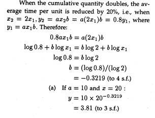
The average time for 20 units if 3.81 hours.
ADVERTISEMENTS:
(b) If a = 10 and x = 30:
y = 10 x 30– 3219
= 3.35 (to 3 s.f.)
The total time for 30 units is 30 x 3.35 = 100.5 hours.
(c) If a – 10 and x = 40
y = 10 x 40-.3219
ADVERTISEMENTS:
= 3.05(to 3 s.f.)
Total time for 40 units is 40 x 3.05 = 122 hours, so the time for units 31 to 40 is 122 – 100.5 = 21.5 hours.
Example 3:
Khaitan Electric Co. has been asked to quote for a new product. Although the company was not involved in the manufacture of the prototypes, similar products have been made by the existing labour force and machinery.
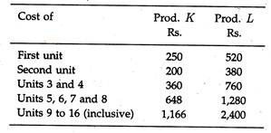
The production records for two similar products, K and L, have been examined and the direct labour costs are summarized below:
It has been estimated that the direct labour costs of the first unit of the new product will cost Rs. 400.
Based on the above information, the learning rate for product K is 0.1522.
You are required:
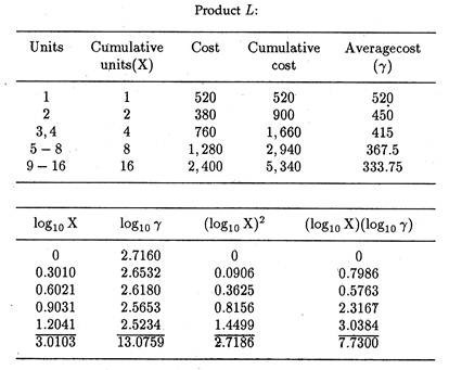
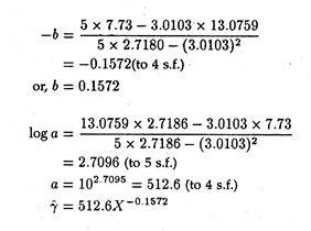
(a) To determine the relationship between the cumulative number of units completed and cumulative average direct labour cost for product L.
(b) To estimate a relationship for the new product.
(c) Using this relationship, to estimate the direct labour cost for a subsequent quantity of 7, i.e., 2 to 8 (inclusive) of the new product.
Solution:
(a) If γ = aX-b
then log10 γ = log10 a – b log10 X
and, therefore, log10 γ and log10 X are linearly related.
(Here γ is the cumulative average cost, a is cost of first unit, X is cumulative units completed and 6 is a learning rate.)
(b) As K and L are similar to the new product, an average learning rate of ½ (0.1522 + 0.1572) = 0.1547 would be used.
When X- = 1, γ = a.
Cost of the first unit is given as Rs. 400. So the relationship for the new product may be estimated to be:
γ= 400 x 0.1547
(c) When X — 8, γ — 400 x 80.1547= Rs. 290 = (to 3 s. f.) Total cost of first eight units = Rs. 290 x 8 = Rs. 2,320.
Therefore, cost of units 2 to 8 is: Rs. 2,320 – Rs. 400 = Rs. 1,920.
Example 4:
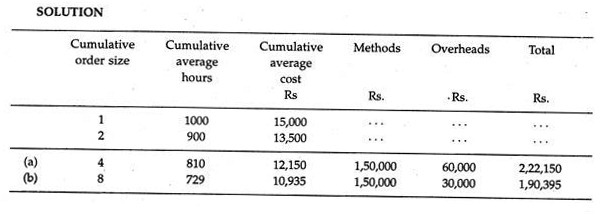
Illustrate the use of learning curves for calculating the expected average unit cost of making:
(a) 4 machines;
(b) 8 machines;
using the data given below: Data.
Direct labour needed to make the first machine 1,000 hours.
Learning curve = 90%
Direct labour cost — Rs. 15 per hour.
Direct materials cost — Rs. 1, 50,000.
Fixed cost for either size orders — Rs. 60,000
Profitability Analysis:
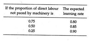
Learning rates may vary from one work process to another. The proportion of labour used in tasks that are not machine-paced is an important determinant of the learning rate.
The following rules of thumb have been developed for estimating learning rates prior to any experience with a new work process:
The rate of improvement in labour efficiency tends to be greater (value of the learning-rate coefficient tends to be smaller) than the above values if the product is a completely new design.
However, if the product is just a modification of an existing one, the initial unit will have labour costs reflecting some of the learning from the previous production run, and subsequent improvement will be smaller (the learning-rate coefficient will be larger) than the values above.
The effects of learning curves upon labour costs make it imperative for new product profitability to be analysed over the whole life cycle of the product. It often becomes necessary to incur losses in early periods, when labour costs are very high, in order to reach those points on the learning curve at which labour costs become low enough that profits can be made.
Example 5:
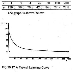
1. (a) Graph the following curve:
y 120x;-0 322
(general form : y = ax–b)
for values of x = 1,2,4,25,50,100 and 200.
(b) Given that:
y – average number of direct labour hours per unit,
a = number of direct labour hours for the first unit,
x = the cumulative number of units produced. Comment on the graph and suggest circumstances in which the use of such a graph would assist in cost accounting. (Assume, for instance, that an order for additional units has already been received).
Solution:
(a) For the given values of x the values of y (to 1 d.p.) are as follows:
(b) y = ax–b is the. equation of a geometric function and as such has the property that its elasticity is constant and is given by the value b. If b = 0.322 then a 1% increase in x will cause a 0.322% decrease in y.
Considering larger changes, if x increases by a factor K, then y decreases to a(Kx)–b, i.e., by a factor K–b. In our example, a doubling of x will cause y to fall by a factor:
2-0.322 = 0.8000 (to 4 d.p.)
If y is the average number of direct labour hours per unit and x is the cumulative number of units produced, then, given an order for additional units which doubles the total number of units produced, the average number of direct labour hours, per unit will fall by 20% as a consequence.
Relevance of Learning Curve in Profit Planning:
The learning curve is often made use of in developing new products and projecting the profitability of such products in the face of rapid technological change. Various other costs such as indirect labour, power, etc. depend on the time required to complete a job.
As learning takes place, these costs tend to fall with an increase in output. As the worker learns from experience lesser and lesser hours are required to finish the same job. Thus, the learning curve theory enables us to predict the average cost at different levels of contemplated output.
This explains why the budget plan should incorporate the effect of learning on costs which, in turn, are related to budgeted volume. At early stages of the production process, the volume of output is usually low. But, with an expansion in this scale of production, the learning effect will gradually become more and more strong.
So, costs will tend to fall. Thus, by taking into account the learning effect over, a budget period, it is possible to forecast company profits.
