The Principles of Effective Demand and Employment Determination | Keynes General Theory

Let us make an in-depth study of the Principles of Effective Demand and Employment Determination:- 1. Introduction to the Principle of Effective Demand 2. Keynes’s Principle of Effective Demand 3. Meaning of Effective Demand 4. Importance of the Concept of Effective Demand 5. Determinants of Effective Demand 6. Determination of the Level of Employment 7. Underemployment Equilibrium and Others.

Introduction to the Principle of Effective Demand:

Prior to Keynes no satisfactory explanation was given of the factors determining the level of employment in the economy.

Economists mostly assumed the prevalence of the state of full employment believing in Say’s law of Markets, an old proposition claiming that all income is automatically spent or that the level of Effective Demand is always enough to lift all goods and services produced off the market.

There were many economists who challenged the assumptions and logic of the Say’s Law. For example, T.R. Malthus tried hard to convince contemporaries the demand in general might fall short of supply in general and the deficiency of aggregate demand might cause general over production and hence general unemployment.

But Malthus failed to explain how effective demand could be deficient or excessive. It was Keynes, who for the first time put forward a systematic and convincing theory of employment based on the ‘Principle of Effective Demand”. The idea behind this theory is not difficult to grasp.

Keynes’s Principle of Effective Demand:

The principle of ‘effective demand’ is basic to Keynes’ analysis of income, output and employment. Economic theory has been radically changed with the introduction of this principle. Stated briefly, the Principle of Effective Demand tells us that in the short period, an economy’s aggregate income and employment are determined by the level of aggregate demand which is satisfied with aggregate supply.

Total employment depends on total demand. As employment increases, income increases. A fundamental principle about the propensity to consume is that as the real income of the community increases, consumption will also increase but by less than income.

Therefore, in order to have enough demand to sustain an increase in employment there must be an increase in real investment equal to the gap between income and consumption out of that income. In other words, employment can’t increase, unless investment increases.

We can generalize and say; a given level of income and employment cannot be maintained unless investment is sufficient to absorb the saving out of that level of income. This is the core of the principle of effective demand.

Meaning of Effective Demand:

Effective demand manifests itself in the spending of income. It is judged from the total expenditure in the economy. The total demand in the economy consists of consumption goods and investment goods, though consumption goods demand forms a major part of the total demand.

Consumption goes on increasing with increase in income and employment. At various levels of income there are corresponding levels of demand but all levels of demand are not effective. Only that level of demand is effective which is fully met with the forthcoming supply so that entrepreneurs neither have a tendency to reduce nor to expand production.

Effective Demand is the demand for the output as a whole; in other words, out of the various levels of demand, the one which is brought in equilibrium with supply in the economy is called effective demand. It was this theory of effective demand which remained neglected for more than 100 years and came into prominence with the appearance of Keynes’ General Theory.

Keynes was interested in the problem of how much people intended to spend at different levels of income and employment, as it was this intended spending that determined the level of consumption and investment. Keynes’s view was that people’s intentions to spend were translated into aggregate demand. Should aggregate demand, said Keynes, fall below income businessmen expect to receive, there will be cut backs on production of goods resulting in unemployment. On the opposite, should aggregate demand exceed expectations, production will be stimulated.

In any community, effective demand represents the money actually spent by- people on goods and services. The money which the entrepreneurs receive is paid to the factors of production in the form of wages, rent, interest and profit. As such, effective demand (actual expenditure) equals national income which is the sum of the income receipts of all members of the community.

It also represents the value of the output of the community because the total value of the national output is just the same thing as the receipts of the entrepreneurs from selling goods. Further, all output is either consumption goods or investment goods; we can therefore say that effective demand is equal to national expenditure on consumption plus investment goods.

Thus, effective demand (ED) = national income (Y) = value of national output = Expenditure on consumption goods (C) + expenditure on investment goods (I).

Therefore, ED = Y = C + I= 0 = Employment.

Importance of the Concept of Effective Demand:

The principle of effective demand occupies an integral position in the Keynesian theory of employment. The general theory has the basic observation that total demand determines total employment. A deficiency of effective demand causes unemployment. The Principle of Effective Demand has its importance on the following counts.

In the first place, it can be said that it is with the help of the concept of effective demand that Say’s Law of Markets has been repudiated. The concept of effective demand has established beyond doubt that whatever is produced is not automatically consumed nor is the income spent at a rate which will keep the factors of production fully employed.

Secondly, an analysis of effective demand also shows the inherent contradictions in Pigou’s plea that wage cuts will remove unemployment. In Keynes’ view, as level of employment depends upon the level of effective demand, wage cuts may or may not increase employment.

Thirdly, the Principle of Effective Demand could explain as to how and why a depression could come to stay. Keynes explained that Effective demand consists of consumption and investment.As employment increases, income also increases leading to a rise in consumption but by less than the rise in income. Thus, consumption lags behind and becomes the chief reason of the gap that comes to exist between total income and total expenditure therefore, in order to maintain effective demand at earlier (or original) level, real investment, equal to the gap between income and consumption, must be made. In other words, employment cannot expand unless investment expands. Therein has the all most importance of the principle of effective demand. It makes clear that investment rules the roost.

Fourthly, it puts the spotlight on the demand side. In contrast to the classical emphasis on the supply side, Keynes placed major emphasis on demand side and traced fluctuations in employment to changes in demand. The theory of effective demand makes clear how and why aggregate demand becomes deficient in a capitalist economy and how deficiency of effective demand generates depression.

Determinants of Effective Demand:

For an understanding of Keynes’ theory of employment and how an equilibrium level of employment is established in the economy, we must know its determinants the aggregate demand function and the aggregate supply function and their inter-relationship.

1. Aggregate Demand Function, and

2. Aggregate Supply Function.

1. Aggregate Demand Function:

Aggregate Demand Function relates any given level of employment to the expected proceeds from the sale of production out of that volume of employment. What the expected sale proceeds will be depends upon the expected expenditures of the people on consumption and investment. Every producer in a free enterprise economy tries to estimate the demand for his product and calculate in anticipation the profit likely to be earned out of his sale proceeds.

The sum-total of income payments made to the factors of production in the process of production constitutes his factor costs. Thus, the factor costs and the entrepreneur’s profit added to them give us the total income or proceeds resulting from a given amount of employment in a firm. Keynes carried this idea into macro-economics. We can calculate the aggregate income or total sale proceeds. This aggregate income or aggregate proceeds expected from a given amount of employment is called the “Aggregate Demand Price” of the output of that amount of employment, i.e., it represents expected receipts when a given volume of employment is offered to workers.

Entrepreneurs make decisions about the amount of employment they will offer to labour on the basis of the expectations of sales and expected profit which, in turn, depend upon the estimate of the total money (income) they will receive by the sale of goods produced at varying levels of employment. The sale proceeds which they expect to receive are the same as they expect the community to spend on their production.

A schedule of the proceeds expected from the sale of outputs resulting from varying amounts of employ­ment is called the aggregate demand schedule or the aggregate demand Junction. The aggregate demand function shows the increase in the aggregate demand price as the amount of employment and hence output increases. Thus, the aggregate demand schedule is an increasing function of the amount of employment.

The question may reasonably be asked: why did Keynes relate expected sale proceeds with employment through output and why not with output directly?

Three possible reasons may be given for this:

(i) Keynes was mainly interested in the factors that go to determine employment rather than output;

(ii) To all intents and purposes employment and output move in the same direction in the short period;

(iii) The total production in the economy consists of a large variety of goods and there is no better measure of it than the labour employed.

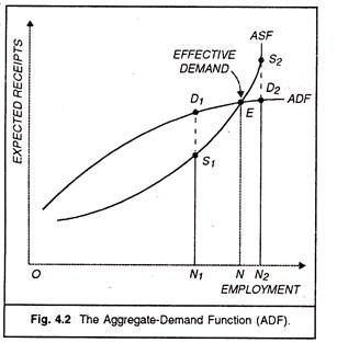
Therefore, if D represents the proceeds expected by entrepreneurs from the employment of N men, the aggregate demand function can be written as D= f (N), which shows a relationship between D and N. The aggregate demand function or demand schedule ADF is shown in the figure 4.2.

We find in the figure that the A Dadoes not start from the origin O because even at low levels of employment consumption will be much above income. As we move along the ADF curve to the right, we find that it is becoming flatter owing to the psychological law of consumption. But the ADF can never slope downwards simply because the absolute amount of consumption in the economy can never go down.

2. Aggregate Supply Function:

Aggregate supply is related to production done by firms. While providing employment to workers, entrepreneurs must feel assured that the output produced by them would be sold out and they will be able to recover their costs of production and get the expected profit margin also. A firm’s output can sell at different prices depending on market conditions. But there are some proceeds of the output for which the entrepreneurs think it will just make worthwhile to provide a certain amount of employment.

The minimum expected sale proceeds of the output resulting from a given amount of employment are called the ‘Aggregate Supply Price’ of that output. In other words, these are the minimum expected proceeds which are considered just necessary to induce entrepreneurs to provide a certain amount of employment. For the economy as a whole at any given level of employment of labour, aggregate supply price is the total amount of (sale proceeds) which all the producers, taken together, must expect to receive from the sale of the output produced by that given number of men, if it is to be just worth employing them.

A schedule of the minimum amounts of proceeds required to induce entrepreneurs to give varying amounts of employment is called the aggregate-supply schedule. This is also an increasing function of the amount of employment. In other words, the minimum sale proceeds necessary go on rising as employment and output are raised. This is due to the rise in cost of production with increasing output, given the capital stock, the techniques of production and organization in the short run.

It is pertinent to observe here that in the aggregate demand function it is the expected sale proceeds that we consider and in the aggregate supply function it is the minimum sale proceeds necessary. There will be difference between them because at certain levels of employment (outputs), producers will expect more proceeds than the minimum sale proceeds necessary. There will be other levels of employment where the sale proceeds expected may be less than the sale proceeds necessary.

The Aggregate Supply Function ASF is shown in Figure 4.2 as rising from left upwards to the right gradually at first and then quickly. The ASF becomes vertical after the point S₂ because at this level of aggregate supply all those who want to be employed get employment. This point indicates full employment in the economy.

Determination of the Level of Employment:

In Fig. 4.2, ADF is the Aggregate Demand Function and ASF the Aggregate Supply Function. We show employment along X-axis and sale proceeds along Y-axis. The point E where the ADF curve is cut by the aggregate supply curve is called the point of effective demand. It may be noted that there are so many points on the aggregate demand curve ADF, but all these points are not effective except point E.

In the diagram, aggregate supply function shows the minimum proceeds which are just necessary to induce entrepreneurs to provide varying amounts of employment; the aggregate demand function shows the proceeds expected from the sale of outputs resulting from various amounts of employment.

Before these curves intersect each other at E, ASF lies below the ADF so that at the one level of employment the expected sale proceeds N₁D₁ are greater than the minimum sale proceeds necessary N₁S₁ showing that the employers will be induced to provide increased amount of employment. At point E, ADF is intersected by ASF’ and entrepreneurs’ expectations of proceeds are realised.

The point E is called the point of equilibrium as it determines the actual level of employment (ON) at a particular time in an economy. The level of employment ON₂ is not an equilibrium level because the sale proceeds expected N₂D₂ are less than the sale proceeds necessary N₂S₂ at this level of employment. Most of the entrepreneurs will be disappointed and will reduce employment.

Thus, we see that:

The intersection of the aggregate demand schedule with the aggregate supply schedule determines the actual level of employment m an economy and that at this level of employment, the amount of sale proceeds which the entrepreneurs expect to receive is equal to what they must receive if their ‘costs’ at that level of employment are to be just covered.

Underemployment Equilibrium:

It may, however, be noted that the economy is no doubt, in equilibrium at the point E, for here the entrepreneurs do not have the tendency either to increase or decrease employment. But Keynes makes a singular contribution to economic analysis by saying that E may or may not be a point of full employment equilibrium. If it is so very good.

If, however, some workers still remain unemployed when ADF and ASF are equalised, in that ease, it will be known as Underemployment Equilibrium. Keynes argued like this. Aggregate demand and aggregate supply might be equal at full employment; this will be so if investment happens to equal the gap between the aggregate supply price corresponding to full employment and the amount which consumers choose to spend on consumption out of full employment income.

Keynes believed that private investment in a capitalist economy is never sufficient to fill such a gap. As such, there is every likelihood that aggregate demand function and aggregate supply function may intersect at a point of less than full employment-called Underemployment Equilibrium.

If underemployment equilibrium is the common situation in the capitalist economy, then how can we achieve full employment 7 Keynes suggested that in the short period government can raise aggregate demand in the economy through public investment which is not profit-motivated.

Refer to Figure 4.3. Suppose the government makes an investment equal to D₂S₂ and this raises the ADF to the level ADF’ and the demand function cuts the supply function at S₂. The vertical line from the point S₂ down on the horizontal axis shows that this policy of public investment would achieve the full employment ON₂ in the economy.

Shapes of the ASF and ADF:

It is very’ difficult to comment upon the shapes of Aggregate Demand Schedule and Aggregate Supply Schedule. Presuming, however, that the money prices of all goods are constant and employment and output rise and fall in proportion to each other, we can safely come to the conclusion that both the aggregate demand function and the aggregate supply function are increasing functions of employment; then rise from left upwards to the right. The ADF rises at first rather steeply and then goes flatter and flatter.

This is because of (nature of the consumption function) MFC being less than one. The ISF rises slowly at first because of the available unemployed resources. As bottlenecks in production are faced, diminishing returns (increasing costs) become more prominent. Beyond the point of full employment, production cannot be increased at all. So the ASF which was rising steeply becomes vertical beyond the full employment point (S₂).

Relative Importance of ASF and ADF Functions:

Since the equilibrium level of employment is determined by the intersection of these two schedules, it would be useful to know some more details about the nature and character of these schedules. Of the two, there is little that is important about Aggregate Supply Function. Keynes gives scant attention to the aggregate supply function and concentrates more on aggregate demand function. For all practical purposes, he takes ASF as given because he deals with the short period and in the short period, supply conditions cannot be changed.

Moreover, in the General Theory, Keynes was concerned with an economy facing unemployment of resources during depression. Under such circumstances, there is little to gain from manipulating the technical conditions of production like costs, machines, and materials through schemes like rationalisation. Rationalisation results in more unemployment in the short period. It was because of these reasons that Keynes took ASF as given.

Since the supply conditions had to be taken as given. Keynes gave more importance to the aggregate demand function. Given the aggregate supply schedule, the resources in an economy would be fully utilised only if there is enough aggregate demand It is because of this that some economists call his theory of employment a ‘theory of aggregate effective demand’. Aggregate demand depends upon consumption and investment. If employment is to be expanded, expenditure on consumption and investment should be stepped up.

Thus, the shape and position of the aggregate demand function depend upon the total expenditure incurred by a community on consumption and investment taken together. Assuming, as Keynes docs, the aggregate supply function to be given, the pith and substance of his argument in the General Theory is that employment is determined by aggregate demand, which in turn, depends on the propensity to consume and the amount of investment at a given time.

Effective Demand Versus Say’s Law:

The classical theory failed in attempting to apply Say’s law to the demand for investment. Whereas it is true that more employment creates more income out of which some will be spent on consumption, the entire increase in income will not be so spent and there is no reason to believe that the difference will be devoted to investment expenditure. Hence if investment does not increase with an increase in employment, the sum of consumption expenditure and investment would be less than the aggregate supply price for the higher level of employment.

Businessmen would reduce employment to a level at which the aggregate supply price exceeds the consumption demand by the actual amount of investment. Hence as long as the gap between income and consumption is not automatically filled up by investment (i.e. Y = C + I) Say’s Law would not operate. It is here that we find Say’s Law uprooted by the concept of Effective Demand as developed by Keynes.

Aggregate Demand in the Statistical Sense:

So far we have considered two determinants of effective demand, i.e., private consumption and private investment, but in modern capitalist societies Government expenditure has also become an additional important item. Thus, Effective demand = C + I + G, Keynes look no account of Government expenditure but post Keynesians treat it as an important constituent of effective demand.

Aggregate demand in the statistical sense is thus made up of:

(i) Private consumption expenditure,

(ii) Private investment expenditure,

(iii) Public investment expenditure,

(iv) Foreign expenditures on domestic goods and services, over and above domestic expenditure on foreign goods and services.

In this way, the aggregate demand is a flow of money expenditure on final output in a given period. All these are components of effective demand.