The following article will guide you about how to show returns to scale on an expansion path.
A rational firm minimises cost by choosing the least cost combination of inputs. This happens in the short run (i.e., at a fixed point of time). However, in the long run a firm may decide to expand its volume of production in order to make more profits or to capture the market by eliminating rival producers (actual and potential).
When a firm or, to be more accurate, its manager decides to produce more, i.e., expand the volume of output, he has to move from one isoquant to another. Since a rational firm (or its manager) is assumed to minimise the cost of producing any level of output, the manager has always to find out an optimum combination of inputs. In other words, when output is to increased, a new least cost combination of inputs has to be found.
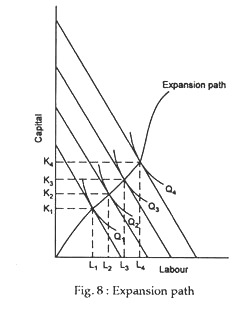
This point is illustrated in Fig. 8, where we see the cost-minimising combinations of the two inputs (capital and labour) for four different levels of output. If the manager decides to produce output Q1, he will have to hire (employ) K1 units of capital and units of labour. Now, if he wants to increase output further to Q3, he will have to use more of both the inputs — K3 units of capital and L3 units of labour.
Thus, every time the manager decides to expand the firm’s output level, he (she) has to spend extra money on the inputs. To be more precise, he has to spend just enough more on inputs to move the isoquant to a point of tangency with the new isocost line. If we connect all of the points of tangency, we obtain the firm’s expansion path. For fixed (market) prices of the two inputs (K and L), the firm’s expansion path is the locus of all cost-minimising combination of inputs.
Thus, as the firm expands its output, it has to move from one point of tangency between an isocost line and an isoquant to another. The firm’s expansion path is the locus of all cost-minimising input combinations.
Returns to Scale:
A firm’s expansion path is used to study what is called returns to scale. Returns to scale describes the relationship between output and proportional increases in all inputs. Strictly speaking, a change in the scale of production of a firm occurs when there is a proportionate change in the usage of all factors. As such, returns to scale is a very important property of the long-run production function.
ADVERTISEMENTS:
When, in the long run, all inputs are variable and are increased, say, in the same proportion, the output can change in one of three ways. First, a doubling of all inputs may lead to an exact doubling of output. In this case, the production function is said to be exhibiting constant returns to scale. Second, a doubling of all inputs may yield more than twice as much output. When this happens, the production function is said to be exhibiting increasing returns to scale. Finally, when a doubling of all inputs yields less than twice as much output we have decreasing returns to scale.
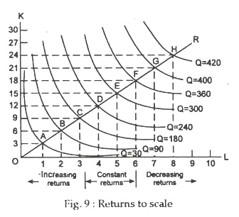
In Fig. 9, we have presented an isoquant map for a production function which shows all the three types of returns to scale — increasing, constant and decreasing. Along the ray, through the origin, factor
proportions (i.e., the capital-labour ratio) remains unchanged. In other words, as we move along that straight line, we increase the inputs in the same proportion.
In this case, we increase capital by 2 units for every 3 units increase in labour, i.e., the ratio of capital to labour is two to three along the straight line through the origin.
ADVERTISEMENTS:
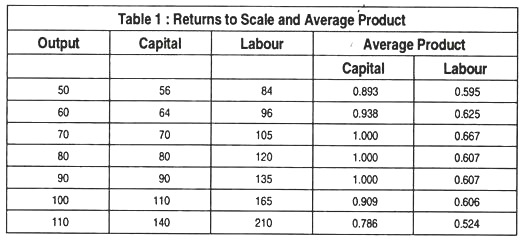
Initially, the production function exhibits increasing returns to scale. As we move from point R to point D, both the inputs rise by 14% and output increases by 20%. Likewise, output rises more than inputs do when there is a movement from D to B. Since output is expanding faster than input usage, the ratio of output to an input, which is the average product, is increasing. As Table 1 shows the average products of labour and capital increase as output rises from 50 to 70.
Further increases in output are associated with constant returns to scale. A movement from B to A indicates that input and output both increase by 14% at the same time. We also find constant returns to scale for output increases up to 90. When this occurs, i.e., when there are constant returns to scale, the average products remain constant.
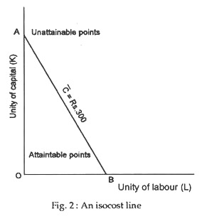
At still higher levels of output, this production function exhibits decreasing returns to scale. In Table 1, as also in Fig. 2, when inputs increase by 22%, output increases by only 11%. This is shown by a movement along the way through the origin from point L to W. Over this range of output average product is falling.
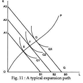
The expansion path shows how factor usage changes when output changes, the ratio of one factor price to another held constant. In Fig. 11 curves Q1, Q2 and Q3 are isoquants depicting a representative production function; A1, B1, A2, B2 and A3 B3 represent the least cost of producing the three output levels. Since the factor price ratio does not change, these isocost lines are parallel.
To derive a firm’s expansion path, we first assume that factor prices remain constant and let total cost outlay, i.e., expenditure on K and L to change. Each equilibrium point is defined by the equality between the MRTS and the factor-price ratio.
Since the latter remains constant, so does the former. Therefore, OP in Fig. 11 is a locus of points along which the MRTS is constant. It is a curve with a special feature — it is locus along which output will expand when factor prices are constant. We may accordingly formulate this result as a definition.
