Break-Up of the Price Effect: 2 Cases

Break-Up of the Price Effect: 2 Cases!

Case # 1. The Hicksian Case:

If the price of one of the goods used by the two-good consumer changes, the price of the other good and his money income remaining constant, then the price effect is obtained. Now, this price effect (PE) can be broken up into the substitution effect (SE) and the income effect (IE) of the said price change. In other words, the PE can be shown to be the sum total of an SE and an IE.

This is because the price of one of the goods and the money income of the consumer remaining the same, if the price of the other good diminishes (increases), then the real income of the consumer also increases (diminishes). Consequently, the income effect of the said price change is obtained upon his purchase plan.

Again, the price of one of the goods remaining constant, if the price of the other good changes, then there is a change in the relative prices of the goods, and as a consequence of this, the substitution effect of the said price change.

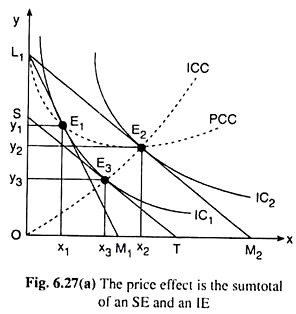
That is why, the price-effect that is obtained because of a ceteris paribus change in the price of a commodity, can be broken up into an SE and an IE. This can be explained with the help of Fig. 6.27(a). By the SE, here it means the Hicksian SE.

Suppose that in Fig. 6.27(a), in the initial situation, the budget line of the consumer is L₁M₁ and his equilibrium point is E₁ (x₁, y₁) on his IC which is IQ. At E₁, the consumer purchases X₁ of good X and y₁ of good Y.

Now suppose, M and p_Y remaining the same p_x diminishes. As a result of this, the new budget line of the consumer would be L₁M₁ and his new equilibrium point would be E₂(x₂, y₂) on a higher IC₁ viz., IC₂.

Therefore, due to the ceteris paribus fall in p_x, the consumer’s equilibrium point would move along the PCC from the point E₁ (x₁, y₁) to the point E₂(x₂, y₂), and the consumer now would purchase x̅₁x̅₂ (or, x₂-X₁) more of good X and y̅₁y̅₂ (or, y₁ – y₂) less of good Y. Therefore,

 

it is already mentioned that this PE is the sum total of an SE and an IE.

Due to the ceteris paribus fall in p_x, two things have happened— the real income of the consumer has increased, and the relative prices of the goods have changed. Now notionally eliminate the improvement in real income by, what Hicks has called, a compensating variation in income, i.e., by an ‘appropriate’ reduction in the consumer’s money income.

Consequently, the budget line L₁M₂ would have a parallel leftward shift and this notional budget line would be ST that would touch IC₁ at the point E₃(x₃, y₃). The tangency between ST and IC₁ indicates that the consumer has been allowed just the initial level of real income—all his real income improvement has been eliminated.

The compensating variation in income (CVI) in this case has been M₂T in terms of x or L₁S in terms of y. The budget line ST represents the change in the relative prices of X and Y, the consumer’s real income remaining constant.

If the consumer is given this budget line his equilibrium point would immediately move along IC₁ from the point E₁(x₁, y₁) to E₃(x₃, y₃). This movement is the SE of the ceteris paribus change in p_x. Due to this effect, the consumer would buy x̅₁x̅₂ (or, x₃ − x₁) more of the relatively cheaper good X and y̅₁y̅₂ (or, y₁ − y₃) less of the relatively dearer good Y.

So it may be written as:

 

The help of CVI is taken in order to isolate the SE-portion of the PE. The consumer may now be given back the CVI amount of his money income, i.e., the improvement in his real income caused by the ceteris paribus fall in p_x may be restored.

As this is done, his money income would increase to the initial amount, prices remaining constant at their (new) L₁M₂ levels. As a result, his budget line would have a parallel rightward shift from ST to L₁M₂ and due to the income effect, his equilibrium point would move along the ICC from E₃(x₃, y₃) to E₂(x₂,y₂).

Due to the income effect, the consumer would purchase x̅₃x̅₂ (or, x₂ – x₃) more of good X and y̅₁y̅₂ (or, y₂ – y₃) more of good Y.

So it may be written as:

Therefore, from (6.38), (6.39) and (6.40), it may be obtained:

So, from (6.38) and (6.41),

SE + IE of the fall in P_x = PE of the fall in P_x (6.41*) is obtained.

It may be concluded from the discussion that the price effect of a change in the price of a good is the sum-total of the substitution effect and the income effect of the said price change.

Case # 2. The Slutsky Case:

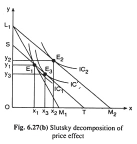
Now come to Slutsky decomposition of the price-effect (PE) into a substitution effect (SE) and an income effect (IE). Rrefer to Fig. 6.27(b). In this Figure, initially, the budget line of the consumer is L₁M₁ and his equilibrium point is E₁ (x₁, y₁) on IC₁.

Now suppose, the price of good X (p_x) diminishes, other things remaining unchanged. As a consequence of this, the consumer’s budget line will rotate from L₁M₁ to L₁M₂ and his equilibrium point would move from E₁ (x₁, y₁) to E₂ (x₂, y₂) on IC₂. This movement represents the price effect of the said fall in p_x.

In order to break up this PE into an SE and an IE, let’s effect a compensating variation in income (CVI) such that the budget line L₁M₂ has a leftward parallel shift from L₁M ₂ to ST. As required by the Slutsky concept of the SE, the line ST passes through the initial equilibrium point E₁. The budget line ST cancels out the improvement in the consumer’s real income caused by the said fall in p_x.

Since ST touches an IC, viz., IC’ at the point E₃ (x₃, y₃) the movement in consumers equilibrium point from E₁ to E₃ represents the Slutsky SE. Now restore the cut in the consumer’s money income due to CVI, his budget line now would have a reverse parallel shift from ST to L₁M₂ and his equilibrium point would move from E₃ (x₃, y₃) on IC’ to E₂(x₂, y₂) on IC₂.

This movement in his equilibrium point represents the income effect of the said fall in p_x. It may very well be seen in Fig. 6.27(b) that the price-effect on the purchase plan of the consumer given by the movement in his equilibrium point from E₁ to E₂ is the sum total of the Slutsky SE given by the movement from E₁ to E₃ and the income effect given by the movement from E₃ to E₂.

The Slutsky SE is under-compensatory as compared with Hicks SE. That is why the SE on the demand for good X would be larger and IE would be smaller in the Slutsky case than those in the Hicks case.