Pricing Policies: Objectives and Techniques (With Diagram)

In this article we will discuss about the Pricing Policies Adopted by Modern Business Firms.

Contents:

1. Pricing Objectives
2. Pricing Techniques in Theory and Practice
3. Pricing Policies and the Interest of the Firm
4. Pricing Policies and Market Conditions
5. Establishing Prices of Related Products
6. Public Utility Pricing
7. Incremental Analysis (Reasoning) in Pricing
8. Going-Rate (Imitative) Prices
9. Customary (Suggested) Prices
10. Pricing Products of Lasting Distinctiveness
11. Economic Theory of Monopoly Pricing
12. Pricing Products of Perishable Distinctiveness
13. Pricing a New Product (or Pioneer Pric­ing)
14. Limit Pricing
15. Retail Pricing
16. Export Pricing
17. Price Changes
18. Cost-Plus or Full-Cost Pricing
19. Product-Line or Multi-Product Pricing
20. Price Forecasting

---

1. Pricing Objectives:

In fact, a study of the pricing objectives of large companies shows that the following are most typi­cal objectives:

i. Pricing to Achieve a Target Return on Investment:

This is a long-term objective and is the most fre­quently mentioned of pricing goals. Under this sys­tem both costs and profits goals are based on stan­dard volume; and the margins added to standard costs are designed to produce the target profit-rate on investment.

ii. Stabilization of Price and Margin:

For some firms, cost-plus is just one step on the road to return-on-investment as a price policy- guide. However, the majority of companies refrain from exploiting products beyond the limit set by cost-plus, either in times of buoyant demand or in pricing different items in the product line.

iii. Target Market-Share:

Some companies have referred to maximum (or occasionally minimum) market-share as a determi­nant of pricing policy. This guide is generally used for products in which the firm does not have a pat­ent or innovative monopoly.

iv. Other Rationalizations:

Pricing to meet or match competition has often been cited as a pricing objective. More often than not, this approach was directed not at meeting competition so much as preventing it.

Dominant companies, cautious of price wars, could justify meeting competition locally on the ground that the policy constituted a permanent threat to potential price-cutters. In other instances, some firms were aware of specific competitive products whose prices must be matched if sales vol­ume was to be expanded.

R. F. Lanzilloti (1958) has pointed out that the large company has a fairly well defined pricing goal related to long-range (planned) profits. It seeks a simultaneous decision with respect to price, cost and product characteristics.

W. Longworth (1964) recommends the use of con­tribution analysis techniques linked with a market-oriented method of price fixing as the soundest base for developing a reliable price-policy.

He sug­gests that “a company will be concerned to fix pric­es to ensure maximum revenue to meet all fixed ex­penses and provide profit. Assessment of product profitability should therefore be concerned on the one hand with those expenses directly related to the products’ manufacture, and variable with vol­ume; and on the other hand to total income result­ing from sales”.

---

2. Pricing Techniques in Theory and Practice:

Though pricing policies are the foundation for the achievement of specific managerial objectives, pricing techniques are to be considered as the tools used in setting or revising prices of individual prod­ucts.

It is generally agreed that actual price should be set on the basis of the interaction of cost, de­mand, and competition. Yet, the pricing techniques used in practice often unduly stress one of these fac­tors to the complete exclusion of others.

The practi­cal problems faced by the business person are im­perfect information, both with respect to cost and to demand, and with the various pricing decisions that have to be made. Another major complication arises due to the existence of a number of institu­tional rigidities that prevent the continuous adjust­ment of prices in accordance with changes in either demand, cost or competitive conditions.

For many products, the price is published in advertising ma­terials or in catalogues and thus must remain un­changed for a long time. For other products sold by large companies, the actual setting of prices is del­egated to many individuals in different settings. Therefore, a system of fluctuating prices would be extremely costly and time consuming.

Pricing executives, therefore, often view the pricing problems as “one of establishing reasonably satisfactory prices for a period of time, rather than selecting the optimum price at a given point in time.

Although the overall objective of establish­ing prices may be profit maximization, the search costs of obtaining information on a product’s cost, demand, and competitive conditions, when com­bined with institutional constraints, may force the decision-maker to proceed toward this objective somewhat differently than is suggested by the static theoretical models”.

Differently put, the decision-maker may know that profits will be max­imized by setting prices according to the marginal rule, but the additional cost of obtaining exact esti­mates of MR and MC may exceed the additional revenue of following this rule, with the result that reliance is placed on simpler rule-of-thumb practic­es.

The actual pricing techniques are designed to assist pricing managers in the establishment of profitable prices. This ex­plains why actual pricing practices are set keeping the marginalize rule of pricing (MR = MC) as the yardstick.

In particular, we will evaluate how cost, demand, and competitive factors guide pricing managers, as well as the interrelationship between pricing theory and actual pricing practices fol­lowed by business firms.

---

3. Pricing Policies and the Interest of the Firm:

From the stand point of the firm, a price policy is intended to maximize long-run profit. This objec­tive is pursued in an environment in which both random events and reactions emanating from other economic organisations have to be taken into ac­count.

The Pricing Process:

According to Alfred Oxenfeldt, there is need to consult (analyse) seven main parties in the process of establishing prices:

Those responsible for sales promotion and advertis­ing;

Consumers of the product;

Existing competitors;

Potential competitors;

Middlemen;

Suppliers;

Government.

One of the major drawbacks of traditional ap­proach is that it focuses almost only on two parties, the buyer and the seller. An actual pricing decision must be based on government rules which force firms to adopt such practices as price discrimina­tion, predatory pricing or collusive pricing.

Thus, pricing has to be viewed as a process that gives sig­nals or information to consumers, competitors, mid­dlemen, suppliers and government.

A Multistage Approach to Pricing:

Oxenfeldt has put forth a multistage approach to pricing that provides a conceptual framework within which to make pricing decisions.

His ap­proach breaks the pricing process into a series of steps, each of which involves specific pricing is­sues:

Selection of market;

Selection of the firm or brand image;

Determination of the marketing mix;

Selection of a specific pricing policy;

Selection of pricing strategy;

Setting specific prices.

In order to select the market target, the firm has to first determine the specific market that it expects to reach and deal with such related issues as market segmentation, market share, competitive advantages, regional markets, and demographic characteristics.

For example, in the soft drink mar­ket, the pricing strategy must reflect unique seg­ments or market categories, such as generic soft drink, low-priced or popular soft drink, costly soft drink, zero-bacteria soft drink, and imported soft drink.

Each segment has different price and income elasticity coefficients and requires a mix of varying advertising and pricing strategies from no adver­tising and low price mark-ups, to saturation pricing and high mark-ups. In a like manner, the pricing strategy may be linked to desired or possible mar­ket share in each segment and in each region.

Likewise, a company’s long-run pricing philoso­phy will be related to the initial decisions made concerning the desired reputation of the product or the firm. Some firms strive to achieve reputations for high-quality products that sell at higher than average prices, while other firms emphasize dis­counted prices. According to Oxenfeldt, price is a variable that must be used to respond to shifting market forces.

---

4. Pricing Policies and Market Conditions:

Price policy has to be examined in the following contexts:

i. Perfect Competition:

A firm can only sell its product at the market price and nothing above it. In the long run, for an ef­ficient firm, the sales price is just equal to the aver­age cost. Normal profit is made. There is no excess profit.

ii. Monopoly:

Monopolies are almost always nationalized en­terprises for which the criterion of maximization of profit is not justifiable. In reality, a firm enjoys monopoly position only because it has succeeded in eliminating or absorbing its competitors. It is therefore probable that, initially, it was better or­ganized and more efficient.

The technical advan­tages which benefit large firms in certain branches of industry can also neutralize, at least partly, the harmful effects of a monopoly. Finally, “any de facto monopoly must be prepared to defend itself, on the one hand, against the emergence of substi­tute competitors and, on the other, against the com­petition of substitute products, which imposes a limitation on its profit realization”.

In general, to prevent the entry of new firms, a monopolist must set entry-preventing prices, i.e., it should hold prices at a level which will tend to discourage new firms from entering that particular branch of industry. This presupposes an implicit es­timation of production costs of possible competitors, and of the profits which will be required to attract them.

On the contrary, in order to fight the competi­tion of substitute products, a monopoly must estab­lish its price policy on the basis of a demand curve which will actually take those products into ac­count.

When the uses of goods produced by a monop­oly are many, the degree of monopoly can vary enormously from one use to another. In case of coal, for instance, sales range from the industrial mar­ket in which the fuel oil competition is extreme­ly active to blast furnace coke market in which coal enjoys a technical monopoly.

So profit maximization demands that manage­ment collect more detailed econometric data in the environment of monopoly, than in that of perfect competition.

iii. Temporary Monopoly:

This situation occurs more frequently. A firm in­vents a new product and places it on the market. For quite some time the demand will remain low, as consumers are not yet aware of the product. The firm will enjoy a de facto monopoly under the pro­tection of its patents.

Then, as the product enters into common usage, demand develops rapidly. Ad­ditional firms try to enter the market. They devel­op new production methods. Gradually, prices and production techniques tend to stabilize. So, at the end, the market evolves towards an ordinary com­petitive one.

A firm which invents a new product must deter­mine a strategy relating to prices and production which leads to a maximum effective income. Fol­lowing J. Dean, we may consider two extreme cases: that of skimming of demand and that of creating a broad market.

iv. Skimming of Demand:

This policy is characterized by very high ini­tial prices and by major promotional efforts. The prices are reduced as the market develops and competitors tend to appear.

The conditions which make such a policy satisfactory are the following:

Firstly, demand is only slightly elastic. This is usually the case when the product is brand new. Consumers are not yet aware of the product or ser­vice and many are drawn by the novelty of the product, all of which contribute to reduce the in­fluence of price.

Secondly, advertising plays an important role in promoting sales. Advertising informs the buyers about a product and excites curiosity.

Thirdly, the elasticity of demand will gradual­ly increase with the passage of time and the firm will progressively reduce its prices. In case of a dur­able good, the policy is one of maximising price to the initial market, consisting of a relatively small number of eager buyers. As the market potential is broadened, the price is reduced to convert potential sales into actual revenues.

Fourthly, if a firm is aware of the fact that it cannot prevent the emergence of new competitors, this policy avoids sacrificing current receipts for less probable future receipts.

Finally, this policy obviates the necessity of making large investments because large-scale de­velopment in the demand for the product is not an­ticipated.

v. The Creation of a Broad Market:

This policy, on the contrary, “is characterized by relatively low initial prices, and consists essen­tially in exchanging present heavy costs against the expectation of future returns”. Certain favoura­ble conditions must exist for this policy to be suc­cessful.

Strong Demand:

Firstly, a strong initial elasticity of demand is needed. This, in effect, permits lowering prices without severely reducing sales revenue.

Large Market Potential:

Secondly, there is need for a large market po­tential. This implies that the product should be potentially attractive to consumers of diverse envi­ronments.

Increasing Returns:

Thirdly, the production process should exhibit increasing returns. In practice, by creating a broad’ market, a firm can avoid working below optimal production capacity and can effect substantial sav­ings in cost.

Entry Prevention:

Finally, there should be some way of minimiz­ing the emergence of new competitors in the mar­ket.

However, these are extreme cases and the price policy must be re-examined periodically.

Imperfect competition:

We have noted that imperfect competition re­fers to markets in between perfect competition and monopoly. There are different varieties of imper­fection: duopoly, oligopoly, monopolistic competi­tion and so on.

vi. Duopoly:

This is the case where there are only two firms in an industry. Each duopolist can choose his pro­duction in such a way as to maximize his income for a given value of output. Each duopolist has no in­terest in modifying his behaviour as long as the other does not modify his.

If both duopolists attempt to take one another’s reactions into account, the problem is no longer pre­determined. Duopoly is often characterised by in­stability.

Duopolists eliminate their competitors through price wars or through agreements. We have already demonstrated that duopolists can as­sure themselves, by cooperating, a total income greater than the sum of the revenues that each can insure for himself by non-cooperative behaviour.

vii. Oligopoly:

In oligopolistic situations, entrepreneurs at­tempt to avoid price wars which are ruinous for the industry. Being aware of the fact that their rivals can do the same, they refrain from seeking to in­crease their share of the market through price cuts.

As a result, oligopoly can attain a certain stabili­ty characterized by:

(a) The ‘price leadership’ of a firm,

(b) The reduction of hidden prices, and

(c) Competition in fields other than that of price (like promotion, packaging, etc.).

Now, about the lowering of hidden prices. It can assume various forms. It is contingent upon the cus­tomer, upon the size of the order, upon the geo­graphical area and the existence of inferior brands. This policy has the advantage that it precedes adjustments of official prices and in this way con­tributes to the stability of oligopolists.

Finally, non-price competition is a substitute for price competition. It is much less dangerous because its effects are felt in the long run. So the possibili­ties of reactions from competitors are more limited.

viii. Monopolistic Competition:

In this type of market, price policies are ex­tremely varied because of product differentiation. Each firm is faced with a separate demand curve and a market price.

---

5. Establishing Prices of Related Products:

There are three stan­dard rules in this context:

The first rule states that the prices of different products must be proportionate to average costs. However, in case of related products, the concept of average cost has no operational significance and can result only from arbitrary agreements. By ap­plying this rule, a firm will be faced with a rigid price policy in the face of changing market condi­tions.

A second rule suggests, on the other hand, that prices should be proportional to short-term margi­nal costs. This rule is more practical since marginal cost can be accurately measured. This rule, as one shall see, is used in case of public utility pricing.

A final rule suggests prices such that profit mar­gins on each product would be proportionate to the value added. However, all the three rules take only cost into account and ignore market conditions.

i. Price Differentiation:

Price differentiation may assume different forms, but the most important are partitioning the market, differentiating prices within a geographi­cal area, and granting discounts to distributors.

ii. Partitioning of the Market:

Dividing a market consist of separating it into distinct sections of differing elasticity. This is the essence of differential pricing or price discrimina­tion.

iii. Price Differentiation within a Geograph­ical Area:

The theory of the economic optimum demands that, at each point, the price of a product will be equal to the sum of the factory price plus a trans­portation cost. However, in order to maximize prof­it, a firm often breaks away from this rule.

In prac­tice, the monopolist charges relatively much higher transportation costs to neighbouring consu­mers than to more distant ones. These policies are found in a somewhat disguised form in the systems used in actual practices which are discussed below.

a. F.O.B. Prices:

This method of rate setting consists in having the consumer pay the sum of the factory delivered price plus actual transportation costs.

b. Uniform Prices:

Under this policy, the same price is charged ir­respective of the geographical proximity of the seller to the buyers.

c. Zone Prices:

Under this policy, the customer is actually billed the sum of the factory delivered price plus a transportation cost but the factory price varies ac­cording to the zone. It is generally lower for distant zones. Zone prices, therefore, constitute price dis­crimination.

d. Parity Prices:

This system “selects a point of parity, the same for all firms. The price scale of a company gives de­livery prices at the parity point. Customers are not charged actual transportation costs but fictitious ones from the point of parity to the point of con­sumption.”

Discounts to distributors:

Trade discounts influence profits obtained by distributors and, if large enough, attract their in­terest. An expanding industry may grant large trade discounts in order to attract a large number of distributors very quickly. These discounts are valu­able in partitioning of markets.

Company price policy is based on economic stud­ies relating to markets, costs, policies of operation, stockage, and investment. True, “price is thus the connecting link between the firm and the outer world: it summaries the demand situation for the firm, and it summarizes for the outside world a firm’s conditions of operation. This intermediary role makes it possible to decentralize the decision function.”

We may now discuss different pricing techniques used and practices followed by modern business firms in both the private and the public sector. We may start with Public Utility Pricing.

---

6. Public Utility Pricing:

Pricing in public utilities such as electricity, gas, water, telephones and public transportation presents a special type of problem. These are ‘natu­ral monopolies’ inasmuch as, in one locality, a single firm tends to drive out competing firms. In these in­dustries, the nature of technology is such that pro­duction and distribution results in substantial econ­omies of scale.

The implication is that one large firm can produce more economically than can sever­al firms. Naturally, the object of government policy is to protect such utility companies from competi­tion and then subject them to rate control by regula­tory commissions.

The Theoretical Basis of Nationalized Industry Pricing:

Many nationalized enterprises are guided by commercial consideration. They seek to maximise profits by setting prices and outputs at levels which make marginal cost and marginal revenue equal. The possible price-output-profit positions for three alternative types of policy of such firms are illustrated in Figure 19.1 for both decreasing and in­creasing cost enterprises.

Where costs are decreas­ing, as in (a), the profit-maximising state firm would produce an output of OQ_p and charge a price of OP_p, earning profits of P_pCDE; the state firm at­tempting to break even, and adopting average cost pricing, would charge OP_a, produce OQ_a, and earn no economic profits; while the firm charging prices equal to marginal cost would charge OP_m, produce output OQ_m, and make a loss of FGHP_m.

In increasing cost industry, as in (b), profit maximising leads to a price OP_p, output of OQ_p, and profit of P_pHJK; break­ing even would lead to a price of OP_a, and output of OQ_a, while the marginal cost pricing firm would charge OP_m, produce output OQ_m, and earn profits of P_mLMN.

Therefore, in a decreasing cost industry, profit maximising results in the highest price and smallest output, average cost pricing produces a lower price and greater output compared to profit maximising, while marginal cost pricing leads to the lowest price and largest output. Marginal cost pricing, therefore, leads to the best use of existing capital but results in a financial loss.

In Figure 19.2, the firm facing demand curve DD₁ has a choice of three plant sizes represented by three cost curves SRMC¹. SRMC² and SRMC³. For each plant size, short-run marginal cost OP3 is con­stant up to capacity output. Long-run marginal cost OP₂ is constant throughout and equal to short-run marginal cost plus long-run capacity cost, i.e. BC.

If plant 1 already exists, the short-run marginal cost price that equates demand and supply is OP ₁, which exceeds long-run marginal cost. If plant 3 exists, then the price charged is OP₃ which is just equal to short-run marginal cost, but is less than long-run marginal cost. With plant 2, price is OP₂ which is equal to both short-run and long-run marginal cost.

Thus, with the right size plant, short-run and long- run marginal cost are equal; if short-run marginal cost exceed long-run marginal cost, expansion of ca­pacity is called for, and if LRMC is greater than SRMC, contraction is warranted. The pricing rule thus also includes an investment rule.

The main argument for marginal cost pricing is that “it relates the cost of producing the marginal unit to the price the consumer pays. This avoids problems of cross-subsidisation and of encouraging consumers to buy excessively goods that are priced below marginal cost, when average costs of produc­tion are rising. Where unit costs are falling, margi­nal cost pricing allows the more intensive use of fixed costs, but brings with it the problem of finan­cial losses”.

Where there are variations in the level of de­mand, either within the day or by the time of year, then marginal cost pricing may be an appro­priate method. For example, in the telephone in­dustry, where demand varies by both time of day and time of year, and short-run marginal costs vary directly with the level of output, it is often argued that the consumer should cover the costs of meeting his demand.

Under such circumstances, pricing the goods or service according to short-run marginal cost is quite inconsistent with long-run marginal cost pricing.

This point is illustrated in Figure 19.3 where the demand and cost curves refer to equal time periods, say of twelve hours, and the equili­brium condition is that the sum of the short-run marginal cost prices should equal the sum of the two-period long-run marginal costs. Thus, night-­time demand for telephone calls (D_n) is charged P_n which is equal to short-run marginal cost or CQ_d.

Daytime demand D_d, given the size of the system must cover the system’s entire capital or capacity cost plus its own short-run marginal cost SRMC. Thus, the price of daytime telephone call is equal to CQ_d plus AC, which is equal to twice the single pe­riod long-run marginal capacity cost (BC). Hence, price can vary between periods and be consistent with the long-run marginal cost pricing rule.

However, this method has certain drawbacks:

Firstly, the price does not cover total cost in a decreasing cost firm. So, the government has to pay a subsidy to the utility so that it can cover all costs. A case is also made in favour of public ownership on the ground that the government is not required to cover all costs out of revenues.

Secondly, if the utility is subject to increasing costs, as is true of telephone companies, marginal cost pricing results in prices which exceed total costs. This result is shown in Figure 19.1. The firm makes excess profit but the size of the profit is less than would be possible without regulation. A spe­cial tax can be imposed to siphon off a large part of the excess profit.

Thirdly, marginal cost pricing is objectionable on the ground that subsidies will have to be pro­vided to utility companies in case of loss. In other words, their profits may depend more upon their success in demonstrating the need for subsidies than in controlling costs. So they may be distracted from their main business if they have to contend with political agencies for subsidies.

---

7. Incremental Analysis (Reasoning) in Pricing:

In a number of business situations there is likely to be a substantial difference between the costs of each on-going business activity on the book of ac­count, and the incremental (extra) costs which de­termine whether or not the activity should be un­dertaken. For various pricing decisions, the incremental costs seem to be the only ‘true’ and rele­vant costs to be considered.

Incremental cost pricing seems to be perhaps the most promising of all the currently utilized pricing tools. It is akin to the marginalist pricing approach inasmuch as it focuses on the impact of changes in output on revenue, cost and profit. However, it dif­fers from the traditional approach because it is more flexible and adaptable in the sense that de­tailed information on demand and supply curves is not required.

Although incremental cost pricing (also known as incremental reasoning) is based on the traditional marginalist principles, it appears to be more suitable for decision-making where con­siderable uncertainty prevails and it is costly to ob­tain necessary information.

The four general guide­lines on which incremental pricing are based are as follows:

If a pricing decision increases revenue more than it does cost, it should be made.

If a pricing decision reduces cost more than it does revenue, it should be made.

If a pricing decision increases cost more than it does revenue, it should not be made.

If a pricing decision decreases revenue more than it does cost, it should not be made.

More simply put, these guidelines suggest that the advisability of introducing any change in price has to be judged by a comparison of cost and revenue changes.

The following four points bear relevance in this context:

1. In making pricing decision, the focus of attention has to be on changes in total revenues and total costs and not on variable cost per unit. Fixed costs (or overheads) have no relevance in incremental decision-making and hence in pric­ing strategy.

2. If we use the incremental approach to pricing in a multi-product firm, we have, of necessity, to bring into focus substitute and complemen­tary relationships. As and when a pricing de­cision for one product affects the sales of an­other product, these effects are to be accorded due consideration.

One of the most glaring ex­amples of a complementary relationship is the concept of loss leader pricing in which the sale of related goods may more than compensate the firm for lost profits. We may consider, for instance, the Hot-Shot camera. It is quite like­ly that this item has been priced below its cost with the expectation that the growing volume of sales of films and bulbs would lead to larger total profits.

In this context, J. L. Pappas and Mark Hirschey have commented that “in addition to the di­rect incremental costs associated with the new product, the firm must consider any impact on the costs of existing products. For example, in­troduction of a new product might cause produc­tion bottlenecks that would raise the cost of other products.”

3. To be able to use incremental reasoning in pric­ing, the manager in charge of pricing must have adequate knowledge about the relation­ship among price, sales volume, and total sales revenue (= P x Q) i.e., price elasticity of de­mand.

4. Finally, where there is substantial idle capac­ity during a fixed period of time, its opportuni­ty cost is zero, and original purchase prices should be ignored. For example, Indian Air­lines may be willing to provide either college students or military personnel transportation at 50% of the original price if it is flying with too many empty seats on a particular route.

A Case Study:

In the early 1960s, Continental Airlines (USA) was trying to decide whether to continue or elimi­nate certain flights in which capacity utilization was very low. As Table 19.1 shows, fully allocated costs reflected the overhead cost of the aircraft purchase price, while incremental costs were based on out-of-pocket costs for labour, fuel and needed maintenance.

On the basis of this information, Con­tinental would increase profits by running the flight because incremental revenues of $ 3,000 ex­ceed the incremental costs of $ 2,000. Fixed costs do not affect decisions because they would be incurred in any case — regardless of whether the flight was made or suspended.

It is to be appreciated that, in such a situation, incremental costs do not determine the price of service, but they can be used to deter­mine the minimum or floor price of $ 2,000, which can be adjusted according to market conditions.

Dif­ferently put, so long as the flight generates $2,000 and no preferable revenue-generating opportunity is in sight, the firm would continue to fly. If there is any improvement in the competitive environment and in demand conditions, higher price can be charged.

Pros and Cons:

Thus, incremental cost provides pricing analysts with an essential guide for short run production and pricing decisions. For example, if a pricing manager is contemplating a reduction in price to raise sales volume, he must know whether the resulting gain in revenue from the additional volume, that is, in­cremental revenue, will exceed incremental cost so as to make net profit positive.

However, incremental costs should not be con­sidered as a major determinant of the price of a product. Instead, they should set a floor and a ceiling within which a wide range of profitable pricing decisions should be made.

The main virtue of the incremental cost analy­sis is that it “involves long-run as well as short-run effects. A new product may appear in the short-run because the firm has excess capacity in its existing plant and equipment. Over the long run, however, this commitment to produce the new item may re­quire a substantial investment when the necessary equipment wears out and must be replaced. There may also be high opportunity costs associated with future production if either expansion of other prod­uct lines, or development of future alternative products, is restricted by the decision to produce the new product.”

The Time Factor in Incremental Analysis:

Time plays an important role in incremental analysis. Business people must recognize that ac­tions taken at one time affect results in future peri­ods. So there may be conflict between short-term profit maximization and long-term profit maximi­zation.

Thus a firm may charge a very low price for its product in the short run and sacrifice some short-term profit to secure larger market share in the long run, and thus maximize its long run profits. Firms also adopt reduced price to prevent the entry of new firms in the industry. This explains why firms do not focus solely on short-run profit maxim­ization.

---

8. Going-Rate (Imitative) Prices:

A simple approach to pricing is to imitate the prices of others. This is usually the case with oli­gopoly firms. But, in practice, the reason for adopt­ing this type of pricing method is not far to seek. It is easy to imitate a rival firm than to take an inde­pendent decision. A firm may get the benefit of an­other firm’s market analysis without worrying about demand elasticities and incremental costs.

It is in the context of ‘going rate pricing’ that the distinction between ‘price takers’ and ‘price- makers’ becomes relevant.

In some markets that closely resemble pure competition, like trading in agricultural commodities or shares and stocks or basic commodities like tin, copper, etc. in the world markets, sellers cannot determine prices but must accept those established by relatively impersonal market forces (i.e., forces of demand and supply).

Such sellers are known as ‘price takers’ — they must take prices as given. But, in practice, such markets are rare. In most markets the sellers are price-makers. They enjoy considerable discretion about prices.

If the primary determinant of price changes is neither cost nor demand, price setting becomes a complex exercise. To be more specific, when the pri­mary determinant of price changes is the competi­tive conditions in the market place, the pricing policy followed by business firms can best be categorized as competition-based pricing.

In fact, price leadership, kinked demand curve, and price-taker models of traditional economics fall within this category of competition-based pricing models.

However, if this pricing strategy is followed, it is not necessary for each firm to charge the same price. Competition-oriented pricing models include not only the prevailing pricing policies and prac­tices in industries dominated by price takers; they also encompass industries in which the price diffe­rentials among firms tend to be maintained over a considerably long period of time.

For example, IBM personal computers are generally more expensive than are Apple or AT&T computers. But this very fact does not preclude the existence of competition- based pricing.

There is one important characteris­tic of this type of pricing policy which distinguish­es it from either demand-oriented or cost-oriented pricing policies: the manager in charge of pricing does not establish a price based on a rigid relation­ship among price, cost, and demand.

Even when costs and demand are subject to change, the firm will make an in-depth analysis of the competitive prices before changing its own price. In other words, the firm will tend to change its price when the competitors do so, irrespective of changes in either demand or cost condition.

The most common type of competition oriented pricing is going-rate pricing. If this pricing policy is followed, the manager in charge of pricing at­tempts to set a price equal to the average price charged by all firms in the industry.

However, adoption of this policy demands a huge amount of information-gathering. Alternatively put, in fol­lowing this pricing policy, the firm’s price would be determined simply by collecting as much infor­mation as possible on all the competitors’ prices and computing their average.

If it is difficult or costly to arrive at an estimate of either cost or de­mand intensity, it is felt that a going-rate price will represent the collective wisdom of the indus­try in terms of yielding a fair return on investment. This pricing policy has the additional virtue that it leads to stability within the industry.

Going-rate pricing policy is mostly followed in industries which produce and sell homogeneous products. However, this technique is not restricted to any particular market structure (like pure com­petition). Instead, it has been utilized both by price takers (e.g., pure competition) and price searchers such as producers of steel (e.g., homoge­neous oligopoly).

The firm operating in a highly competitive environment acts as a price-taker (as in monopolistic competition in the long run) simply because it has hardly any choice. By contrast, firms operating in highly concentrated industries are constantly monitoring the prices charged by ri­val producers.

If there is the slightest price differ­ence among these firms, the firms charging the lower price will gain at the expense of others by being able to attract most of the customers. The ri­val firms are thus forced to quickly match the low­er price for fear of losing sales.

In industries where firms produce differentiat­ed products (as in monopolistic competition or dif­ferentiated oligopoly) managers in charge of pric­ing enjoy more discretionary power in pricing decisions. The reason is not easy to find.

In such markets, non-price considerations (such as product, price, service) influence the buyers in purchasing products. In such situations, the pricing manager frequently seeks to place his product within a range of acceptable prices with respect to those charged by rival firms (or competitors).

For exam­ple, although Air India does not charge exactly the same prices for its services as do all of its com­petitors (such as JAL, PAN AM, BRITISH AIR­WAYS, THAI INTERNATIONAL, LUFTHANSA, etc.) the very fact that the air express industry has become highly competitive in recent years has led Air India to fix its price, keeping in view a range of prices charged by these numerous competitors.

However, the major drawback of this pricing strategy is that it does not guarantee profit- maximization by firms. Secondly, a pricing policy which is adopted by following current competitors may make the industry stagnant and attract new firms into the industry.

---

9. Customary (Suggested) Prices:

Sometimes, managers just follow suggested pric­es of manufacturers or wholesalers. This practice gives them enough time to devote to other deci­sions. But what is a suggested price? It is probably the one “that the manufacturer or wholesaler has found feasible under the market conditions and thus permits the retailer to gain the benefit of market analysis without having to engage in it.”

This pol­icy has one drawback: it limits flexibility in meet­ing local conditions. But it is attractive to those sellers who prefer to escape the pain of analysing those conditions.

In the case of retail price maintenance (RPM) the retailer hardly enjoys any freedom. He (or she) has to sell the item only at the price established by the manufacturer. Such practices protect some retailers from unfair competition from large out­lets. Moreover, some manufacturers apparently pre­fer the control and stability of price that RPM pro­vides.

Statutory Pricing:

In recent years it has become common for many governments to operate some kind of price policy, as part of an anti-inflation strategy. This may take a variety of forms, but usually involves the setting of some limit on permissible price increases. Some­times a legal minimum price is set. If the minimum price is set below the equilibrium level, excess de­mand is likely to emerge.

So the firm’s freedom of decision-making is considerably reduced. The opti­mum price is set within the legal or institutional constraints. For the firm introducing a new product in a period of anti-inflation policy, it is also im­portant to ensure that the original price is set cor­rectly where demand exceeds supply. But it may be difficult or impossible to raise it sufficiently to avoid losing potential profit.

One strategy to avoid inflation control is to re-­launch the product in slightly different form, so that a new price can be charged. Generally, howev­er, decision-makers conform to the law. This raises ethical questions and leads us to the whole question of social responsibility of the firm. Increasingly, firms set prices to earn less than maximum profit, or to stabilise employment, investment etc.

---

10. Pricing Products of Lasting Distinctiveness:

Joel Dean has drawn a distinction between:

(1) Products of lasting distinctiveness and

(2) Prod­ucts of perishable distinctiveness.

In reality, we hardly come across products of lasting distinctive­ness, if “lasting” means more than ten years, and “distinctiveness” means absence of close (accepta­ble) substitutes. In theory, it is often possible to es­tablish a strong monopoly position in a single prod­uct.

But in practice, the existence of excess profits inevitably encourages outsiders (potential compe­titions) either to develop substitutes or to imitate the original product.

One of the important sources of monopoly power is the control of scarce mineral deposits like tin or copper. But, in such cases also, the monopoly position of a firm is constantly chal­lenged by new discoveries of ore that can be profit­ably mined at the going price.

Dean has also cited the examples of metallurgical and chemical progress which “have found entire arrays of substi­tute materials that displace monopolized metals at various price levels”. Moreover, “Patents have also proven a shaky barrier to competitive entry”.

In a number of industries it is found that “inadequa­cies of patent protection make it more profitable to pool technical advances among firms than to try to exploit additional discoveries”.

So it is safe to pre­dict that a new product which is distinctive at the outset will inevitably degenerate, over the years, into an ordinary (common) commodity with the en­try of new firms into the industry. The pricing of such short-lived specialities will be discussed in the following section.

To start with, it is worthwhile to examine at the theoretical level long-run monopoly pricing. By pure monopoly “we refer to a company whose products’ substitutes are so distant and scattered that its sales depend on its own price level and on economic conditions, but are not affected by prices of any particular group of sellers”.

No doubt, the company’s price level may affect the actions of sub­stitute competition. But such actions only affect the marginal buyers slightly.

---

11. Economic Theory of Monopoly Pricing:

We have already dealt with the simple ana­lytics of monopoly pricing. Recall that the demand schedule for the distinctive product of the monopo­list is shown in revenue functions: average revenue and marginal revenue.

We have also shown the be­haviour of corresponding costs: average cost and marginal cost. The whole thing boils down to find­ing the price and rate of output that will maximize profits.

The simple theoretical analysis provides a clue to practical pricing. It points out the kinds of de­mand and cost relations that need to be guessed and shows how these functional relations should be used to indicate the most profitable price.

However, a major qualification of the usefulness of such analysis is the restraint on profit maximi­zation as a pricing objective. So the above solution is highly over-simplified and difficult to apply.

In fact, for the pure monopoly situation, there are complex econometric problems of estimating the de­mand and cost curves. The analysis also fails to take into account potential competition and the re­actions of substitute competitors and their effect on future prices. In practice, these are vital factors in most monopoly pricing problems.

i. Statistical Problems:

Our simple approaches to monopoly pricing re­quire usable estimates of demand and cost. Monopo­ly pricing raises tough problems in the field of de­mand analysis. In a competitive situation, demand analysis is based on the narrow range of relevant prices. In fact, in the long run, the general level of prices is set by cost conditions in the industry.

So, no sales are possible above the selling price (and no individual company’s actions are especially impor­tant). On the contrary, the monopolist enjoys con­siderable discretion in setting prices, and identify­ing the best possible price calls for estimates of the effect of price-volume over a wide and dubious price range. Such estimates can be made with sta­tistical methods, survey questionnaires and con­trolled experiments.

In general, the elasticity of demand is estimat­ed to be lower in the short run than in the long run. In the short run, price increases evoke consumer re­sistance. It reflects the consumers’ decision to go without the commodity. But, in the long run, consu­mers get necessary time for adjustments.

So they switch to substitutes as prices increase. Similarly, demand is more responsive to price cuts in the long run than in the short. These responses depend on “cultural lags, on the amount of capital investment needed to take full advantage of the new price, and on the rate at which substitute competition is ex­cluded from the market as prices fall”.

However, all theoretical demand curves have a major pitfall: wherever the time period under con­sideration is short, they cannot take account of the full range of reactions to price changes, in terms of speculative buying and to substitute improvement.

Any price change has a tendency to stir up inquiries and new ideas about the monopoly. This is why most monopolists prefer to maintain stable (rigid) prices for years together than to maximize short run profits.

In a like manner, since the monopolist’s equili­brium depends as much on demand elasticity as one cost conditions estimation of future cost behaviour is equally vital. Such forecasts require knowledge of a host of factors such as rate of output, sale of plant, prices of resources and, of course, technology. All are embodied in the functional relation of cost to operating conditions.

These forecasts also require “projections of these operating conditions them­selves”. We have already examined the tech­niques of cost estimation and of forecasting. How­ever, obtaining such estimates is an expensive affair.

Moreover, these cost curves are relatively transitory. They keep on shifting their positions continuously. So they fail to tackle the problem of projecting into the future the operating conditions themselves.

As Dean has pointed out, “The practical pricing problem of a monopolist is usually to find a price that he can keep for long periods under varying conditions of demand. This calls for cost forecasts that cover a range of factor prices, and even encom­pass some technical progress and product improve­ment”. So, the theoretical solution to the monopoly pricing problem has little relevance for any real case of long run monopoly.

ii. Potential Competition:

It is important to take note of potential compe­tition when long run monopoly is provisional-rather than permanent. The source of such monopoly may be striking innovations (e.g., nylon or punched card accounting).

It may spring from “an accumulation of technical or selling superiorities, where, once hav­ing gained the bulk of the market, the company can make the most of large-scale economies in produc­tion, distribution, and research, to hold off poten­tial competition.”

In this context Dean has cited the example of General Motors.

In fact, the de­mand curve for the provisional monopolist must reflect two things:

(a) The entry of high-cost mar­ginal producers in response to higher prices and

(b) The possibility that new competitors can beat the large-scale economies presently enjoyed only by the monopolist.

Cost and profit estimates are vital for applying this long-term pricing criterion in quantitative terms. The relevant cost here is “the cost to a poten­tial new entrant working at the current price level and using the available technology”.

The relevant profit is the entrants’ prospective rate of return on investment. And the investment relevant here has to encompass, in addition to investment in produc­tion facilities, investment in cumulative advertis­ing, and in distribution arrangements required to compete effectively.

Dean has pointed out that, in most industries, the important potential competitor is a dominant, multi-product firm operating in neighbouring indus­tries.

For such a competitor, the most important con­sideration for entry is not the profit margin being enjoyed by the existing monopolist but the prospect of large and growing volume of sales. Such firms can reduce costs per unit by producing more. So what is significant is the relationship between price and their estimate of their own potential cost.

iii. Substitute Competition:

In practice, substitute competitors react directly to price changes by changing their own prices. One can ignore the possibility of substitute competition so long as the distinctive product is only a minor competitor to each of its substitutes. But in practice, the change in the price of a product affects the de­mand for its substitutes so strongly that price changes of substitutes become necessary.

We can cite the example of aluminum which competes directly with copper on a price basis, for use in electrical cable, where the important consideration is cost per unit of capacity. But price is only one of the various factors in aluminium’s competition with steel and glass for structural and cooking purposes.

Dean has noted that “when there are close com­petitors on price for some uses of the product, the demand curve is to this extent indeterminate unless reactions of substitute rivals can be forecast”. This is the basic problem of oligopoly.

In truth, there are few distinctive products, however distinctive, then can ignore rival’s reactions entirely. For exam­ple, drug manufacturers, in pricing a new product, must consider the possibility that old medicines thereby made obsolete, will resist displacement by reducing price down to their incremental cost.

---

12. Pricing Products of Perishable Distinctiveness:

The product (or service) offered for sale by a firm forms a link between itself and the consumer (and society at large). Until the last century (or at best the pre-World War II period) the rate of tech­nological changes or product innovation was so slow that product-competition was neither very stiff nor widely varying.

The initiator (or the company first offering a superior and differentiated product) enjoyed a period of partial monopoly position until its rivals imitated it. But that took too long a time. However, things have now changed. Today, an in­novation gives the innovating company a decisive cost or quality advantage of just what may be called perishable distinctiveness.

The initiator in­deed can increase the sale of his product at the ex­pense of its rivals and may be by successive innova­tions (technological upheavals.) But this shortens the life cycle of the product.

Each product, in general, has a life-cycle, i.e., it passes through different phases over its life­time.

A typical life-cycle has four distinct phases:

(1) Product launch (or initiation stage),

(2) Growth phase,

(3) Product maturity and

(4) Decline phase.

A company’s pricing policy for its product needs to be related to all the phases. For the analysis of pricing in the early stages of the product — when the product first appears in the market — is signif­icantly different from that in the later stages, when the product is suffering from imitations, (i.e., competitive encroachment from new products) as well as from shifts in taste.

In the initial stage, the seller’s price discretion is wide, as the product is the pioneer’s ‘speciality’, but, as the distinctive speciality fades over time into a pedestrian ‘com­modity’, the sellers’ market it with interdepen­dence in price-decision as the principal market strategy.

It is thus not surprising that Dean should argue: “Continual changes in promotional and price-elasticity and in costs of production and dis­tribution throughout the cycle, call for adjustments in price policy”

---

13. Pricing a New Product (or Pioneer Pric­ing):

“Pricing problems start when a company finds a product that is a radical departure from existing ways of performing a service, and that is temporar­ily protected from competition by patents, secrets of production, control of a scarce resource or by other barriers”.

There are two kinds of (pricing) policy for a new product:

(1) A skimming price policy, with initial high prices (sometimes coupled with heavy promotional outputs) that creams off the top of the market; and

(2) A penetration price policy, with low prices at the beginning acting as an acces­sory for mass market penetration from the very out­set.

A skimming price policy is employed by the pro­ducer of a new product when the demand for the product (in the short run) is relatively inelastic, since high prices will not deter high-income pio­neer consumers. The demand is inelastic because the product is new (sharply differentiated from previ­ous products) so that the scope of price comparisons and substitution is limited.

Moreover, a high price creates usually an aura of ‘quality image’ for the largely untried product because purchasers are prone to judge quality by the price (indeed, heavy rate of promotional activity has to be deployed for making public aware of the new availability). Dean is of the view that skimming price helps the firm to cover costs, and thus it is a safer road to tread.

In the initial stage, high price will make it possible to recoup initial R&D expenses, heavy promotional expenditure and plant investment, and will serve to offset the high costs of producing on a small scale which is inevitable in the early stages.

Price is likely to be most important at the early stages of introduction in cases where the product has no more than a small degree of novelty. If there are no close substitutes, price may well be a secon­dary factor at the early stages of introduction to the market. The product pioneer, as Joel Dean pointed out, has a choice between two basic strate­gies.

Skimming Price:

Here he takes advantage of any price insensitivity which exists at the early stages of market­ing and charges a high ‘monopoly’ price. This ena­bled him to secure a relatively high cash flow at an early stage which helps to minimize his losses if, in the end, the product fails to ‘take-off. If, however, demand builds up according to his hopes and expectations, then he will be earning high re­turns.

According to Dean, price skimming refers “to the practice of setting the price of new product at a rel­atively high level upon its introduction to the market, and, in effect, “skimming the cream” from the market. The product will be purchased only by those consumers who are willing to pay the initial price in order to have the product sooner rather than later”.

Sometime after the product is intro­duced at this relatively high price, effective de­mand will begin to fall and the market will gradu­ally get saturated, indicating that the supply of consumers willing to pay that price is diminishing. The decision maker may then decide to lower the price of the product in order that the next-most- eager section of the market can be induced to buy it.

In Figure 19.4, we suppose that price was ini­tially set at P_t and that sales at this level accumu­lated at Q_t. If we assume that the same demand curve remains appropriate in future, and if price is then slashed to the level indicated by P_{t + 1}; sales in this later period will total Q_t+ 1 units. In a later period, perhaps, the price may be lowered to P_t + 2 and sales will increase to q_{t + 2}.

This type of pricing behaviour is often treated as second degree price discrimination. In this case, consumers are discrimi­nated among on the basis of their willingness to wait for the product to become available at a lower price.

A historical example of this pattern of price adjustment has been provided by ball-point pens, which now retail for a mere fraction of their intro­ductory price. More recent examples include com­puters, electronic calculators, VCRs, VCPs and quartz digital watches.

The opposite strategy is adopting the policy of pricing at a very low level to penetrate the mass markets early, where these markets consist of buy­ers who are unwilling to pay a high premium for the novelty or speciality of a new product.

To elab­orate the point a little more, the low-price pattern should be adopted with a view to long-run rather than short-run profits, with the recognition that it usually takes time to exploit the full potentialities of the market.

Thus this opposite strategy has the aim of dis­couraging competition. This strategy is usually fol­lowed when the producer feels that the period of exclusive occupation of the market is likely to be of short duration. Competition will arise quickly and his aim is to try to make this as unattractive as possible by setting a low price and a good margin of profit.

The conditions for penetration pricing are:

(1) Lower elasticity of demand in the short run than in the long run,

(2) Economies of scale in production,

(3) The threat of new substitutes and

(4) A favoura­ble impact on sales of the product under considera­tion, over the sales of other company products, and on customer goodwill.

In choosing a particular strategy of pricing skimming or penetrating — the firm might well consider the price of substitutes. A skimming price is justified if prices of substitutes are also high or if substitutes are too remote to be worthy of considera­tion.

However, a penetration price policy may be adopted by a firm in the growth stage of its product — management may lower price in order to ‘bring the product within reach of a sizeable market and so initiating the growth of the mass market’.

At this stage, elasticity of demand will be higher and the price-conscious buyers will now arrive at the market to buy it; the firm can expand sales consid­erably by lowering price, and in doing so it can gain the economies of large-scale production.

Again, in the face of new or potential entry into the market by competitors, the pioneer firm may capture and maintain a large share of the market by adopting a low penetration price policy. The initiating firm must bring its price in line with its competitors’ as the latter’s products make the pioneer’s one less characteristically distinctive enough to command a price premium.

Pricing Mature Products:

There are certain symptoms which can indicate the maturity stage of a product:

(iii) Weakening of brand preference;

(iv) Narrowing of physical variation among prod­ucts;

(v) Market saturation; and

(vi) Stabilisation of production methods.

As the product matures (‘speciality’ converts into ‘commodity’ only), losing its distinctive char­acteristics, and with several substitutes well esta­blished in the markets, the prices of all these tend to fall in line with one another. Attempt on the part of any firm to slash its product price will pro­voke nothing but price-wars.

To avoid this, some form of price-leadership will be the ideal institu­tional set-up, the company with the largest mar­ket share usually adopting the role of the price leader. Thereafter, competition will be on the ba­sis of ‘promotion, advertising, and minor product improvements’.

---

14. Limit Pricing:

Joe S. Bain has introduced the concept of limit or staying-out pricing. He has pointed out that when an existing firm — be it a monopolist or an oligopo­list — is making a positive economic profit, it may decide to set the price below the profit-maxmizing level in order to reduce or eliminate the possibility of the entry of new firms into the market. So limit pricing may also be called entry-preventing pric­ing.

Limit pricing is used to project long-run profits of an existing firm. The concept is illustrated in the diagram below. In Figure 19.4, D and MR are the ex­isting firm’s demand (average revenue) and margi­nal revenue curves, respectively.

Its short-run aver­age and marginal cost curves are shown by SRAC_E and SKMC_E. Here OQ* is the profit-maximizing level of output and OP* is the corresponding price. The long-run average cost curve of the industry is LARC.

Since there is excess profit in the short run, new firms can join the industry at the scale represented by SRAC_N and make some profit at the prevailing price OP*. However, existing firms may realise that they can make the size of profits greater if they succeed in preventing entry.

But this requires sacrifice of some short-run profit. Thus, the existing firm may set a lower price and still make a posi­tive economic profit. But this action would prevent entry. P₀ is less than SRAC_N at all levels of output.

A new firm contemplating entry into this indus­try must realize that “even if the existing price were high enough to permit them to earn a profit, entry may not be desirable. If existing firms main­tain their current levels of output in the face of ad­ditional competition, price can be expected to fall.”

As the demand curve in Figure 19.5 above shifts to the left due to entry, the current level of output of that firm, OQ*, could be sold only at a lower price. However, if entry causes price to fall below the level represented by the minimum point of SRAC_N, a new entrant would incur an economic loss.

Pricing for a Rate of Return:

In the 1920s, D. Brown, the then vice-president of General Motors, U.S.A., developed a pricing for­mula which is based on an average sales estimate or “standard volume”.

The overall pricing objective was to determine a standard volume large enough to cover fixed costs and variable production costs at price customers were willing to pay, while still permitting the firm to earn a target return on capi­tal employed. Brown contended that the pricing objective was to obtain the highest rate of return on capital consistent with attainable volume.

A popu­lar pricing method commonly called target return pricing has been developed on the basis of his ide­as. The object of the firm is to determine a target- return price, which is equivalent to determining the necessary profit per unit sold that will permit achieving the target return if actual demand equals forecasted demand.

However, such an ap­proach ignores the differences in capital invest­ment required to produce various products. Some in­vestment, e.g., in materials, is more current and requires a different rate of return. To tackle the problem of different types of capital, contribution analysis is helpful.

Target Returns Pricing:

Target return pricing refers to a set of product prices designed to provide a predetermined return to capital employed in the production and distribu­tion of the products involved. In this pricing meth­od, both costs and profit goals are based on stan­dard volume.

Standard volume “is the volume or quantity expected to be produced in the following year, or an average volume expected to be produced over a number of future years”.

For an expected vol­ume, the firm determines what its unit labour and materials costs must be, and allocates its fixed costs over the expected volume to obtain a figure of aver­age fixed cost. To these standard costs is added a percentage of capital employed per unit volume to arrive at a selling price. In equation form the pric­ing rule is

PR = DVC+ F/X + rK/X

Where P_r = selling price determined when the target return formula is used

DVC = direct unit variable costs

F = fixed costs

X = standard unit volume

r = profit rate desired

K = capital (total operating assets) employed.

Pros and Cons:

The effect of target-return pricing is to help pre­vent cyclical or seasonal changes in volume from unduly affecting sales prices. In other words, the firm expects that averaging the changes in cost and demand over seasons or business cycles will enable the firm to realize a desired rate of return on in­vestment.

However, as in full cost pricing, pricing decisions based on this approach are not at all re­sponsive to demand or shifts in demand. Like full- cost pricing, target-return pricing provides the needed stability in making pricing decisions, since standard volume and standard costs are usually based on expected volume over a planning horizon.

However, it almost ignores price competition. Yet this approach is adopted because of management’s increasing concern with allocating scarce capital resources over various alternative uses.

To illustrate the appreciation of this method, assume the data given in Table 19.4. From this data, the selling price of each product can be ob­tained using Eq. (1).

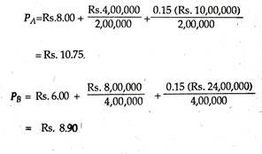
Table 19.4 summarizes the data for each product for the purpose of comparison. If the company makes only these two products, A and B, and the expected volume of the product-mix is realised, the target return is achieved. However, this approach ignores a number of factors, which may result in one or both products failing to achieve the desired re­turn.

Disadvantages of the Target Return Approach:

First, this approach assumes that the product sales mix will remain in a fixed (2:1) proportion, ignoring market acceptance of the formularized prices. However, acceptance of a product line’s prices depends on price differentials within the line as well as the price differentials with competitive offerings.

Thus, the prices as formularized may not lead to the desired rates of return. For example, if actual sales volume, at these prices, is 180,000 units for a and 400,000 units for B, then the return on cap­ital for A is only 9.5%, and overall, the firm will have a rate of return of 13.38%.

A second difficulty is that mark-up is based on fully allocated costs. A full-cost approach, as we have noted in the preceding section, distorts the ef­fects from shifts in activities or demand. Indeed, no out-of-product costs were incurred, and it is not pos­sible to analyse the effect on contributions, of set­ting lower prices.

Finally, the approach assumes that each prod­uct in the product line carries capital investments in the same proportions. So, it makes no distinction in production costs between materials cost and con­version cost. However, materials—intensive product is likely to require relatively more capital investment than a product for which the major proportions of costs are for conversion.

---

15. Retail Pricing:

The extent to which retailers will wish to handle a firm’s goods will obviously depend on the profit margin available. The mechanism for achieving such profit is the trade discount system. Retailers’ profits mainly come from being able to make a margin over the cost of buying goods, to­gether with cost associated with selling them.

The difference between the cost price (i.e., the price to the retailer) and his selling price is known as the “gross profit margin.” If we deduct selling costs from this margin we get the “net margin”.

In the words of Gough and Hill, “The normal method of quoting price to the retailer is for the manufacturer (or wholesaler) to state a recommended selling price for the goods and then deduct the trade dis­count — in effect; this suggests the gross profit mar­gin. Whether this is the actual gross profit margin, depends on policy over selling prices — if the man­ufacturer is able to control selling price then the trade discount is the gross profit margin to the re­tailer.”

This practice of selling prices is known as “resale price maintenance”. However, it has now largely vanished. Instead, the retailer sets his own selling price and hence determines his own gross profit margin.

Thus, in most normal situations the manufacturer (or wholesaler) cannot control the profit margin of the distributor, and because of this has greater difficulty in controlling the num­ber and type of outlets for his goods. The price which is quoted by the manufacturer is merely a suggested or recommended price.

How does this affect the retailing firm? The standard marginal analysis may be adopted for the typical retail outlet. This is illustrated in Fig­ure 19.9.

Here AR is the demand curve for the product. MR is the corresponding marginal revenue curve. On the cost side, there are two important elements: the cost of the good bought from the manufacturer, and the associated selling costs (sales, clerical workers, rent, insurance etc.).

Suppose there are quantity discounts, i.e., by purchasing more, the re­tailer can buy at a lower cost. In this case, the cost of an extra unit falls as the number of goods pur­chased rises. This may be called the “marginal buying cost curve” (MBC) and here it is assumed to fall linearly.

On the selling cost side, it is assumed that cer­tain factors are fixed in the short run (size of pre­mises, fleet of delivery vehicles etc.) while others, like the number of sales staff, are variable. True, a certain amount of staff is necessary before the busi­ness can function at all, but this level of staff can cope with a significant increase in retail trade be­fore extra staff have to be called in.

Therefore, the marginal selling cost curve (MSC) can be expected to fall significantly at low levels of output, and more gradually thereafter. Sooner or later, a stage may come where the increase in staff combined with the given fixed factors tend to lead to decreasing re­turns, and hence to a rise in the MSC curve at high sales level.

The marginal cost curve MC is derived by adding MSC and mbc curves. Profit is maximised at sales of OQ’ and a price op’, because at this point MR = MC.

The gross trading margin at this level of sales will be determined by the difference between average revenue and average buying cost (abc), in Figure 19.9. The net trading margin will be set by the difference between average revenue and average total cost (ac) at this output level by the vertical distance.

So long we have focussed mainly on the costs of the retail outlet and paid little attention to the suggested selling price quoted by the manufacturer. However, suggested or recommended prices have in practice been used by retailers to advertise “dis­counts” to the customer of that particular store.

Thus, the practice of« “double-pricing”—quoting a recommended price and then an “own” price—may have a marked effect on the demand curve. In par­ticular, people may be more motivated to buy a good at a price of Rs. 150 discounted to Rs. 125, than if it is simply priced at Rs. 125.

Thus, the advertising effect of double-pricing may be considerable. It shows that “in these cir­cumstances, pricing and advertising may be comple­mentary rather than alternative strategies for the firm.” Again, “in these circumstances, distributors have a motivation towards wanting a high recom­mended price from the manufacturer, in order to quote a high saving or discount for the customer.

If distributors are able to bargain with manufacturers in this way then the nominal gross margin between suggested selling price and cost price may be very wide, although the actual gross margin will be con­siderably less.

So the conclusion is that the distributive margin is a highly complicated issue involving both dis­tributors and manufacturer. In most real life situa­tions, the ability of the manufacturer to control the number and type of retail outlets is often only par­tial and sometimes very weak indeed.

---

16. Export Pricing:

Export pricing is an example of differential pricing — charging of different prices for identical goods or services when supplied at different times and/or to different customers. Price differences are often based on geographical (spatial) differences.

The barriers created by space are perhaps greatest when firms are selling in different countries. There is ample evidence that, despite some reluctance to ‘subsidize the foreigner’, prices tend to be lower in export than in domestic markets, because of the greater competitive pressures in the export market.

Most firms set about the pricing process for ex­port sales in much the same way as for home sales, but experience greater competitive pressure on ex­port prices. More firms are opposed to the setting of prices in the home market which does not fully cover direct costs plus a full contribution to over­heads. However, in export pricing, most firms are prepared to consider such prices.

In foreign trade, two types of prices are used: f.o.b. and c.i.f. F.o.b. is an internationally accepted abbreviation for free on board, indicating that the stated value of goods includes all costs up to the border of the exporting country, and that these in­clude loading charges at the border. F.o.b. valua­tion can be used to value both imports and exports.

C.i.f. is an abbreviation for cost insurance freight, indicating that the stated value of goods includes all costs up to the border of the importing country, and that these include loading charges at the border of the exporting country and the costs of insurance and transportation to the border of the importing country. C.i.f. valuation usually applies only to imports.

---

17. Price Changes:

It is of interest to examine the circumstances in which a price change may be initiated, particular­ly after a period of good trading at a given price. In fact, if conditions of cost or of demand change, then a firm, in any type of market situation, will adjust price and output in order to maximise profit.

i. Cost Changes:

The main factor leading to a price change is change in cost. The original price of most products is based on costs. So rising costs lead to rise in pric­es. Moreover, the price-cost relationship does change during the life cycle of any product. In prac­tice, certain cost factors do change at the same time but in different directions.

Thus “the initial devel­opment costs may have been fully recovered or the productivity of the manufacturing processes em­ployed may have increased”. Since price increase is not always feasible (may be due to consumer re­sistance or government intervention) businesses of­ten try to offset some pact of increases in raw mate­rial prices or wage costs by a more efficient use of resources.

However, if cost of raw materials and wages are rising rapidly as in a period of inflation, off­setting economies will be insufficient and price in­creases must occur.

In such a situation, and in the absence of government controls, competitors are all likely to raise prices quickly and by much the same amount. Any drop in sales is likely to be spread over competing firms, not uniformly, but in a way which most will find tolerable.

Price changes are never welcomed, though ris­ing prices due to rising costs encounter least resent­ment. On the contrary, if raw material prices drop by 10% but, after a time lag, the price of the prod­uct drops by only 5%, accusations of profiteering will almost certainly be heard.

ii. Demand Changes:

Price changes may also come from the demand side. A price may have been set to skim off a high- income segment of the market and this policy may be implemented. The price may subsequently be brought down to attract new market segments.

This is observed in case of seasonal fashion goods or even seasonal fruits and vegetables. Prices are set high at the beginning of the season. At some future date, when it is felt that this market is fully satis­fied, prices are reduced to clear stocks.

iii. Activities of Competitors:

If a firm is in a monopoly position such as a pharmaceutical firm (with patent protection for a drug which is in widespread use) it can charge a big ‘skimming price’ and make monopoly profits. If a rival is likely to enter the market, the monopo­list will, in all likelihood, reduce his price drasti­cally with a view to making the business unprofit­able to the rival firm.

iv. Price Leadership:

Finally, in oligopoly, a dominant firm often acts as a ‘price leader’, initiating changes of price which are followed by other firms in the industry. For the followers, a price change is a reaction to events rather than a thought-out strategy.

---

18. Cost-Plus or Full-Cost Pricing:

For firms in the unreal world of perfect competi­tion, no price policy would be possible. However, in the real world of imperfect competition, the mar­ginalist rule of profit maximization cannot be ap­plied because the notion of demand and supply curves for a product loses its precision. The knowl­edge of the businessman regarding his demand and supply curves is inadequate.

How then does the businessman actually fix the selling price of his product? The answer to this question was first suggested by R. L. Hall and C. Z. Hitch (1939). They developed the concept of full- cost or cost-plus pricing. Most business firms usually use the ‘full cost’ principle, that is, they charge a price based upon full average cost of production, in­cluding a conventional allowance for profit.

This is also known as mark-up pricing. The effect of compe­tition is to “induce firms to modify the margins for profits which could be added to direct costs and overheads, so that approximately the same price for similar products would rule within the ‘group’ of competing producers.”

How is this price arrived at? According to Hall and Hitch, this price is likely to approximate to the full cost of the representative firm. In other words, this price is reached directly through the community outlook of businessmen, rather than in­directly through each firm working at what it’s most profitable level of output would be if competi­tors’ reactions are neglected, and if the play of competition varied the number of firms.

Therefore, the price set should cover the costs incurred in efficient production and allow reasona­ble margin of profit. The process of calculation, of course, varies. The price fixer may calculate the average direct costs of producing an article. To this he will add a ‘costing margin’ or the margin of gross profit on the article. It includes indirect or overhead cost and the net profit earned.

Since, however, the costing margin in a multi-product firm may vary from one product to another; it dif­fers from the realized gross profit margin as shown in the trading account. Alternatively, a profit mar­gin is added to full cost, that is, average direct cost of production plus an allocation of overhead costs.

The object is to play safe by covering cost and adding a margin of profit. But for this the product must sell in sufficient quantity at that price to re­alise expectations.

The position is illustrated in Figure 19.10. Av­erage direct or variable costs are represented by OA.

We put fixed cost on this. The ATC curve is downward sloping for obvious reasons. For sales volume ON, the average fixed cost is AB. To OA plus AB is added the desired unit net profit CB, to arrive at a selling price OC.

Clearly this will work out only if the market will take ON units at this price. If no more than ON₁ units can be sold in the market, costs are covered but no profit is earned. If sales fall below this point the product loses money. This may occur in a dynamic market.

Price Stability:

This full-cost price has a tendency to be stable in the long run. It will be changed if there is a sig­nificant change in labour and raw material costs, but not in response to marginal or temporary shifts in demand.

P.S.W. Andrews (1949) made the following ob­servations in defence of full cost pricing:

The price usually quoted for a particular prod­uct will equal the estimated average direct cost of production plus a costing margin.

The costing will normally cover the costs of the indirect factors of production and provide a normal level of net profit, looking at industry as a whole, and may reflect any general permanent changes in the prices of indirect factors of production.

Whatever the level of output, price will tend to remain unchanged so long as the prices of direct fac­tors of production do not change.

At that price, the business will have a more or less clearly defined market, and will sell the amount demanded by its customers, its sales thus equalling its limited share of the market for its product(s).

Figure 19.11 illustrates the concept of average (full) cost pricing. A price-maker will plan to sell OM per period at a price of MP per unit. This price is set by taking its average direct costs of produc­tion and adding a costing margin.

Traditional microeconomics postulates that the costing margin, AP, depends upon the assumption that the firm knows the cost and demand for its product and attempts to maximize profit. In the full-cost analysis, the costing margin may be AP, or it may be adjusted to approximate towards AP by trial and error.

If the firm is unaware of the cost and demand Conditions for its product, or pursues any other objective rather than to maximize profit, the costing margin may differ.

In practice, very few business pursue goals other than profit maximization. When they have other objectives, such as security, the extent to which these are achieved will vary more or less directly with the profits earned. They can abstain from the maximization of profits due to difference in expec­tations about the behaviour of demand and cost, or in the extent to which they look to the future.

According to the full-cost principle, businessmen seek to maximise net revenue by varying the size of the costing margin in the light of their expecta­tions of demand. Certainly, according to the margi­nal analysis, the price of a product responds solely to changes in the price of the direct and indirect factors.

The full-cost principle operates to protect firms against the possibly disastrous effects on profits produced by the existence of surplus capacity in an industry which is fairly competitive and whose products are fairly competitive. The pricing deci­sions of some small business show the application of the full-cost principle.

Drawbacks:

The cost-plus-method has four major draw­backs:

There is the problem of defining precisely what is the true total cost of making and selling a prod­uct.

A second problem arises because most indirect costs are fixed in the short run and do not vary with output.

Thirdly, a fixed market ignores the influence of demand.

Finally, it ignores the competitive structure of the market within which the firm operates.

W. Haynes has pointed out that these defects can be removed, at least partly, by applying a flex­ible costing margin. Some firms set their prices in relation to the price set by the large firm or firms in their industry. Thus, retaliation by more power­ful competitors is avoided. This expedient of ‘go­ing-rate pricing’ again transfers some of the em­phasis in pricing from cost to the market.

Cost-Plus Pricing — as a Synonym of MR = MC:

It apparently seems that cost-plus pricing is a straightforward contradiction of the MR = MC rule. It appears to ignore demand totally, and makes no concession to competition — actual or threatened.

Furthermore, it involves circular reasoning. If vol­ume sold depends on price (as it does in demand analysis) but price depends on cost, (as in cost-plus pricing) then how can price be determined, since cost depends on volume sold (as it does in cost anal­ysis)?

However, a close scrutiny shows that busi­nessmen choose a mark-up which they deem ‘neces­sary’ or ‘appropriate’ and so the paradox is resolved. There is no conflict between the accoun­tant’s rules of pricing and the economic point of view.

Recall that in profit maximization, MR = MC.

Thus, the left hand side of this expression (the mark-up under cost-plus pricing) is higher the less elastic is demand and vice-versa. The more price elastic a product is, the lower is its mark-up. Thus cost-plus pricing can simply be a synonym for MR = MC.

Competitive Bidding (Tendering):

Finally, cost analysis is essential in many pric­ing situations where the product is built to customer specifications and the production contract is awarded to the lowest qualified bidder.

Bidding situations are probably the most fasci­nating type of pricing problem, particularly when the nature of the product is such that the marginal production costs are significantly less than the win­ning bid.

Many technical products (involving engineering skills) and construction projects (involving utilisa­tion of equipment that might otherwise stand idle) are sold by the submission of sealed bids. Here the bidder’s objective is to quote a price which is slightly lower than the lowest competitive bid, thus winning the contract at the highest possible price.

Two approaches are possible in arriving at a competitive bid. A demand analysis is theoretical­ly appropriate. But, in practice, rather than esti­mating the quantity that will be sold at each pos­sible price, the bidder would estimate the likelihood of winning the contract for each of a range of possible prices.

At a price just above varia­ble costs, the chances of winning might be 100%; at a very high price the chances would always be nil. The best price would be one which maximised the bidder’s expected profit, using probability theory as described in decision theory.

---

19. Product-Line or Multi-Product Pricing:

i. The Nature of the Problem:

Most companies produce a number of products at the same time. So product-line pricing is an impor­tant practical problem for most companies. Since most companies make several related products, product-line pricing is an important phase of price policy.

And “the key economic feature with respect to the pricing of a company’s product line is the na­ture of the interrelated demand for parts of the firm’s input, which, when measured in quantita­tive terms, takes its most common form as cross- elasticity of demand”.

Multiple products are produced for two reasons: either because:

(1) The demands for the various products are related, or

(2) Production costs are lower when products are jointly produced.

Keeping this in mind, we may note some implications of product-line pricing under two separate conditions, viz., where goods are substitutes for each other, and where they are complements.

In the words of M. H. Spencer, “The overall problem in product- line pricing is to manipulate the combination of prices until the optimum or most profitable price structure is achieved”. In the opinion of Dean, “The problem of product-line pricing is to find the proper relationship among the members of product group”. This problem also arises when the products give the seller an opportunity to charge different prices.

Dean has cited the following cases:

(1) Use-differentials (e.g., fluid milk versus cheese milk),

(2) Seasonal differentials (e.g., morn­ing movie specials), and

(3) Style-cycle (e.g., print­ed shirts).

If the goal is to price the new product so that it “fits into the line” in a consistent manner, cost-price ratios for the existing products may be a valuable pricing guide.

Because of the inter­relationship of the various items in the line, the demand curves for the individual products may be strongly influenced by the prices of other items in the line that are either substitutable or comple­mentary; the products are subject to “cross- elasticity” of demand. The relevant demand curve for a group of related products is, of course, the curve for the entire product line.

Another type of product-line problem arises when traditional price classes exist for the quality-range of items offered. Familiar examples are women’s fashion wear, automobiles and gasoline.

Product costs are very important in such situations because the manufacturer can rarely charge an un­conventional price — Rs. 1,000 for a car is unheard of. Rather, the pricing decisions is made by decid­ing to produce a product which will sell in one of the established price classes.

The optimal price is the one that equates marginal revenue to marginal cost. Usually, marginal revenue is more or less con­stant, and it is marginal cost per unit that changes radically, increasing at higher volumes of output.

ii. Pricing of Substitutes:

A firm produces substitute goods in an effort to segregate consumers or market sectors with differ­ent elasticities, in order to profit from the different taste idiosyncrasies. Spencer had cited the follow­ing examples of firms producing competing (substi­tute) products: meat packers, automobile manufac­turers, fire companies, clothing producers, cigarette firms, soap companies and pharmaceutical houses.

The producers of these products compete with themselves because they produce products to fill similar needs. The more they sell of one product at any given time, the less they may sell of others.

There are two different methods of product-line pricing for substitute goods. Firstly, a mark-up method of pricing may be used for the whole range of products with the same margin employed for all similar products in the line. The common technique is to price the products in proportion to costs.

Secondly, a product may be priced by varying the size of the margin with the level of costs. It follows, therefore, that the more costly the product, the higher the margin, and, hence, higher the price.

In short, the objective of the product-line price structure is to exploit the differences in demand elasticities between market sectors that yields the maximum ‘contribution margin’, tempered by ex­pected secular shifts in demand and by competitive forces such as market share and possibility of entry by new firms.

iii. Pricing Complementary Goods:

When two goods are used jointly we have de­mand interrelation of a complementary type. We can think of cameras and film, stereo phonographs and records, or Dettol and Dettol Soap where the ultimate product being sold is ‘physical hygiene’.

There are three pricing strategies for such goods. These are discussed below:

1. Loss leaders:

This refers to the sale of a commodity at less than invoice cost or at a price sharply below custo­mary level, and publicizing the fact through ad­vertising. This is mostly-practised in retailing.

The intention is twofold, viz.:

(1) To draw in customers who would buy other products and/or

(2) Create cus­tomers’ interest which will ultimately shift the demand curve to the right.

In most cases, complementarity reveals a time dimension between present and future demand. A firm expects that present losses will encourage fu­ture sales and profits, e.g., trial subscriptions for magazines, student rates on block purchase of art film tickets etc.

In some cases, the complementarity is between different products at the same time (e.g., Nescafe coffee and chocolate) and the direct losses to the loss leader (e.g., on chocolate) are more than offset by the indirect gains in the complementary goods (e.g., on coffee).

2. Tie-in sales:

This practice requires buyers to combine other purchases with their preferred goods, so that in ef­fect, the seller is offering the purchaser a joint product. For example, Texmaco Ltd. can compel tex­tile manufacturers to purchase other materials and intermediate goods as a condition of purchasing textile machinery.

3. Two-part tariff:

Here the buyer pays two prices for a joint prod­uct. For example, we have to pay a fixed amount for telephone wiring and a variable amount depending on use.

The object here is to cover initial costs with fu­ture income to be derived from the variable service (e.g., the minimum charge for telephone services and the variable payments for extra calls made). This is mostly practiced by public utility concerns.

Note that the primary object of product-line pricing is to evolve an appropriate structure of product prices. But the ultimate object is to manipu­late the price structure until the desired combina­tion of prices for reaching the desired end is achieved.

Each price structure will produce a different sales mixture and, therefore, a different combina­tion of total revenue and total cost. Therefore, “the optimum price structure is one that produces the greatest expected difference between total revenue and cost, or in other words, the largest expected net profit”.

---

20. Price Forecasting:

All the methods used for demand forecasting may also be used for forecasting the market price that will exist in the next (or some future) period. We would use some kind of a qualitative forecast. Or, we might use a time-series in which price fol­lows a trend.

However, in practice, we normally use an econo­metric model to obtain market price forecasts. This requires that we specify and estimate both the market demand and market supply functions.

After estimating these functions, we must obtain the forecasted values for the exogenous variables (e.g., income and prices of inputs.) Inserting those forecasts into our estimated demand and supply functions, we can solve the equations to obtain the price forecast. Consider the following hypotheti­cal example.

Suppose the manager of Reliance Ltd — a manu­facturer of clothing — was preparing the firm’s production plan for the first quarter of 1996. One of the firm’s divisions produces moderately priced men’s shirts and the manager wanted to obtain a price forecast for his product for 1996 that would subsequently be used in making the production deci­sion for this division.

The manager realized that in this particular segment of the shirt market, Reliance was only one of many firms that produced a fairly homogeneous product and none of the firms in this moderate price shirt market engaged in any significant advertis­ing. Hence, this market approximated closely the conditions of a perfectly competitive market.

Therefore, the manager specified a simplified de­mand supply system for the market:

Demand: Q_t = a + bP_t + cY_t

Supply : Qt = e+fP_t + gP_F,t

Using quarterly data for the period 1991 to 1995, these equations were estimated.

The estimat­ed demand and supply functions were as follows:

Demand: Q_t = 125 -2P_t +12.5Y_t

Supply: Q_t = 250 + 8P_t + 5P_Ft

In this estimation, sales (Q) were expressed in thousand units, the price of the product (P) in ru­pees per unit, and income (Y) and price of factors (P_f) in Rs. ‘000.

To obtain 1996 forecasts for the exogenous varia­bles, the manager purchased forecasts of income and input prices from a large econometric firm. The 1996 forecast for the price of inputs was Rs. 10,000. So, in the model, the forecasted 1996 value for P_F was 10.

However, in the case of an income forecast for 1996, the forecasting firm provided three different forecasts, each based on different assumptions about government policy changes.

These income forecasts were as follows:

High = Rs. 22,000

Best = Rs. 18,000

Low = Rs. 14,000

In forecasting the price of shirts in the first quarter of 1996, the manager of Reliance would then have three alternative values of Y _1996I. 22,18 and 14.

To obtain price forecasts for shirts, it was neces­sary for the manager to insert the forecasted values for the exogenous variables into the estimated de­mand and supply functions. Using the high forecast for income one gets:

Demand : Q_1996I, =125- 2P_1996I+ 12.5(22)

= 400 – 2P_1996I

Supply : _Q1996I = 250+ 8P_1996I +5(10)

-200 + 8P_1996I

Establishing an equilibrium, i.e., setting quanti­ty demanded equal to quantity supplied,

400 – 2P_1996I = 200 + 8P _1996I

Solving this equation for price,

P_1996I = 20

Hence, the manager of Reliance Textiles found that the 1996 forecast for the price of shirts, assuming the high-income forecast, is Rs. 20 per shirt.

Exactly in the same way, using the best income forecast for income in 1996_I, the forecasted price of shirts in the first quarter of 1996 would be Rs. 15 per shirt. And, using the low-income forecast, the 1996 price forecast would be Rs. 10 per shirt. So, the manager of Reliance Textiles has three price for shirt for the first quarter of 1996:

High = Rs. 20

Best = Rs. 15

Low = Rs. 10.

---