Pricing in Theory (With Diagram)

The below mentioned article provides an overview on Pricing in Theory.

Market Analysis:

Price determination occupies the central stage of economic analysis and of managerial decision mak­ing as well. It is because price affects demand or quantity sold, and quantity sold in turn affects cost. Thus, price affects profit through its effect on both quantity demanded (and thus, total revenue) and total cost. Hence, pricing a product is a strategic decision-factor in planning for profit.

Though in general terms we refer to demand and supply as the forces behind the price of a commodity, in prac­tice, there are other factors as well: government policy, objective of the producers, market structure (i.e., nature of competition) and so on.

The determination of price and (thus, output level) is very much dependent on the competitive structure of the market. This is because the firm op­erates in the market, and its decision-making vari­ables are affected by its environment. The phrase competitive structure refers to the nature and extent of the monopolistic elements, if any, that may be present in any particular market structure.

The chart below depicts economists’ classifica­tion of markets on the basis of competitive condi­tions:

We may classify the nature of competition ac­cording to two aspects of market structure:

(1) The number of sellers, and

(2) The degree of product dif­ferentiation.

Purely Competitive Firm and Industry:

A perfectly competitive market has the follow­ing features:

(a) A large number of buyers and sellers:

A single buyers or seller has almost no influence on the mar­ket price, because any one’s share in the market is very small.

(b) Homogeneity of products:

The product of any seller is identical to that of any other in the market.

(c) Free entry and free exit:

Any individual or company is free to enter or leave the commodity market in the long-run.

(d) Perfect knowledge:

All buyers and sellers have perfect knowledge about the market for the com­modity so that there is no room for uncertainty.

(e) Indifference:

No buyers has a preference to buy from a particular seller, and no seller has a pref­erence to sell to a particular buyer.

(f) Independence:

Collusion among sellers is com­pletely absent.

(g) Scale of activity:

Each producer is assumed to experience constant returns to scale.

Under such a market each firm acts as a price- taker; and it can have no price policy. Price is deter­mined for all firms producing an identical commod­ity by the interaction of market demand and sup­ply curves. An equilibrium price prevails for all the firms in the industry. The demand curve facing an individual firm in this case is thus, perfectly elastic, i.e., horizontal.

At the market-determined (equilibrium) price, the firm can sell all it wishes, but nothing at a higher price. Each firm will adjust its output so that margi­nal cost is equal to market price (or marginal rev­enue, as in this case demand curve is perfectly elas­tic).

In the short-run, a firm may earn super-normal, profits since price may be greater than the average cost for the output level; and a firm may also incur loss if price is less than average cost.

However, in the long-run free entry (in the case of super-normal profits) and free exit (in the case of loss) of firms will make the firms move to a position where price will equalize minimum average cost (also equal to marginal cost). At the long-run equilibrium, each firm will earn only normal profits. The optimum output will, however, be different for different firms de­pending on cost conditions.

We can derive the equilibrium conditions of a firm under perfect competition as follows: For profit maximisation, MR = MC is the usual con­dition. Again, since e_p is infinite, AR = P = MR (i.e., horizontal demand curve), and the first-order condition becomes

Figure 18.1 illustrates the price and output de­termination of a firm under perfect competition. At the market determined price OP, the firm’s average revenue or demand curve (AR = MR) is D₁ D₁. Now, the first-order condition (MR = AR = MC) is satis­fied at two points X and Y.

But at X, the slope of MC curve is negative. But at Y, the second-order condi­tion is satisfied. Thus, at the equilibrium point, MC curve must intersect the MR curve from below. The firm under consideration makes profits equal to the area of the (shaded) rectangle AD₁YZ.

A change in market demand curve (from D₁ D₁ to D’₁D’₁) would cause a change in market price (from OP to OP’), industry output (from OQ to OQ’) and the output levels of various firms in the indus­try (in our case, from OQ₁ to OQ’₁). Profit would increase or decrease depending upon the nature of shift.

A Numerical Example:

We can illustrate the same short-run adjust­ments using a numerical example. In table 18.1, six different market prices are assumed. When the mar­ket price is Rs. 61, we know that the demand and marginal revenue curves that the firm faces are per­fectly elastic at Rs. 61.

The firm would then produce 10 units (MR = MC = Rs. 61) and earn an economic profit of Rs. 120. At a market price of Rs. 46, the firm maximizes profit where MR = MC = Rs. 46, and produces an output of 7 units.

Since TR = TC at 7 units, there is zero economic profit. When market price falls to Rs. 41, the firm reacts by decreasing its output to 6 units (MR = MC = Rs. 41), and at 6 units it incurs a loss of Rs. 30. The firm will continue to produce in the short-run until price falls below Rs. 35 because the minimum point on the AVC curve is at Rs. 35.

To see why, examine the adjustment when market price falls to Rs. 32. At Rs. 32 the firm would produce 4 units, but if it does, it losses Rs. 72. (TR = 4x Rs. 32 = Rs. 128; TC = 4x Rs. 50 = Rs. 200; and Rs. 128- Rs. 200 = -7.) If it shuts down, the firm loses only Rs. 60 in to­tal fixed cost, as the total variable cost (TVC) would have been Rs. 140 if production had taken place. (TVC = 4x Rs. 35 = Rs. 140; TFC = Rs. 200- Rs. 140 = Rs. 60).

So it loses less if it stops pro­duction. At any price less than Rs. 35, the firm will shut down or close down its operations completely.

Suppose a competitive firm in the short-run can sell all its output at a fixed price of Rs. 10 per piece. Given the cost function (in Rs.) of the firm

C = 2q³ – 24q² + 80q + 85.

What is the profit maximizing output level?

What is the maximum amount of profits?

Do you think that the firm will produce any­thing in the present situation?

Solution:

C = 2q³ – 24q² + 80_q+ 85

So, MC = dC/dq 6q² – 48q + 80

For equilibrium

P = MC, i.e., 6q² – 48q + 80 = 10

or, 6q² – 48g + 70 = 0

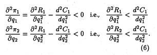
Solving for q, we get q = 6.1 or 1.92 (approx.) Again, the second-order condition is:

d_2π/dq² = 0-d²C/dq²˂0,i.e d²C/dq²˃ 0.

So, at 6.1 units output level, the firm will attain its equilibrium, i.e., its profits will be maximised.

Again, π = R-C = 10g-(2q³ – 24q² + 80q+ 85)

So, at q = 6.1, π — 10 x 6.1 —[2(6.1)³ —24(6.1)² +8(6.0) + 85] = -72.92 (in Rs.).

So, maximum profits amount to a loss of Rs. 72.92. Hence, the firm will not produce anything since it is losing at the profit-maximizing output level. And the firm cannot improve upon its profit level, by influencing its product-price.

Figure 18.1 (b) represents the situation of a com­petitive profit-maximising firm in short-run equilib­rium. In the short-run, the firm in question is earn­ing super-normal profit.

But, if the firm faces a de­mand curve like DD in Figure 18.2(a) below, lying below AC curve but above the AVC curve, the firm would only be able to cover part of its fixed costs, for at Q, average fixed cost is AC (the difference be­tween AC and AVC curves). But, the firm would continue production in the short run, even if it in­curs loss of AB per unit of production.

In fact, when its demand drops to the level indi­cated by the line D’ D’, which touches the AC curve at its minimum E, the firm would lose all its super­normal profit. Instead, it would only cover its costs. This is the break-even point for the firm. How long can the firm go on?

Only up to the point where the demand curve D” D” touches the AVC curve. The point is termed as the shut-down point. Beyond this point the firm cannot operate even in the short- run, since the firm has to cover at least its variable expenses.

Thus, the firm in the short run would produce up to the point where the demand curve intersects the rising portion of the MC curve, i.e., MC curve becomes the supply curve here. But not the whole of it. Rather, that portion of the MC-curve, lying above the AVC_min, i.e., SS” in Figure 18.2(b) above, is the supply curve.

But firms, if they were making losses in the short run, cannot continue indefinitely in that po­sition. Some firms would leave the industry. That would reduce supply and as a result price would rise. The demand curve would rise to a position D’D’ as in Figure 18.2(a).

If they were making super-normal profits, new firms would enter the market, thus increasing the overall supply and re­ducing price. The demand curve would go down to D”D” position. Thus, in the long run, a firm would be at equilibrium at the point £, i.e., the AC_min , where we have

AC = MC = MR = AR.

This is a no-profit, no-loss position, where all the firms are said to earn only normal profits.

Monopoly Pricing:

Monopoly is a market situation which is dia­metrically opposite to that of perfect competition. There is a single seller/producer, without any rival producing any close substitute for the monopolist’s product.

The monopolistic firm itself is, therefore, the industry. The demand curve facing a monopo­list possesses the same properties as the industry de­mand curve for a perfectly competitive market. This is, q =f(p) is the demand function, where dq/dp < 0.

It may be noted that, unlike an individual firm, the monopolistic firm is the price maker and can in­crease his sales only by cutting price. A perfect com­petitor adjusts his output level for a given (industry) price level in order to maximize profit.

But a mo­nopolist is at liberty to vary either output or price to reach an equilibrium, but not both at the same time. A monopolist would be expected to have U-shaped AC and MC curves. Then the equilibrium situ­ation would be as shown in Figure 18.3.

The equilibrium of a profit-maximizing monop­olist will occur at the point where MR — MC, and MC curves cuts MR curve from below.

Thus, in figure 18.3, E is the equilibrium point, OP is the equilibrium price, OQ is the equilibrium output, and the shaded area PSTA represents the volume of total profit. Monopolists arrive at the same conclusion about their production using marginal costs and marginal revenues as they do using total costs and total rev­enues.

Figure 18.4 graphically represents some hy­pothetical data. We observe that the profit-maximi­zing level of output of the firm can be identified graphically, both as being the highest level reached before the MC rises above the MR, and as the level at which there is the greatest gap between total costs and total revenue. See Table 18.2.

Monopoly Profits are Not Inevitable:

Figure 18.5 depicts a situation in which profits are possible when the demand for a firm’s prod­ucts would be depicted by a downward sloping de­mand curve. But profits are not inevitable even for a monopoly, at least in the short run. Monopolists may have costs and revenue conditions that result in temporary losses or normal profits.

There are three possible profit alternatives for a monopoly (hypothetical situation). Having a mono­poly does not guarantee profits. Whether or not there can be profits depends upon whether or not there are customers who will pay prices high enough to exceed production costs.

Most public bus services in India rim at a loss. Figure 18.5 represents the three basic alternatives (winning, losing, staying in the game) that might occur for a monopolist.

Long-Run Equilibrium:

Long-run equilibrium adjustment for a mono- ply firm takes one of two possible forms:

(1) If the monopolist incurs a short-run loss and if there is no plant size that will result in pure profit (or, at least, no loss), the monopoly will go out of business; or

(2) If it suffers a short-run loss or earns a short-run profit with the original plant, the manager must determine whether a plant of a different size (and thus a different price and output) will lead to a larger profit.

If the latter course of action is followed, the firm will adjust the plant size in such a fashion that the output at which the new marginal revenue equals long-run marginal cost, can be efficiently produced.

This point is illustrated in Figure 18.6. The mo­nopolist would build a plant to produce the quan­tity at which long-run marginal cost equals marginal revenue. In each period, Q₁ units are produced. Av­erage cost is OC and price per unit is OP₀ .

There­fore, long-run total profit is CP₀BE. This is the maximum profit possible under the given revenue and cost conditions. In contrast, the monopolist op­erates in the short-run with the plant size indicated by SAC₁ and SMC_1.

Monopoly and Perfect Competition Compared:

In general, monopoly price is higher than com­petitive price and monopoly output lower than com­petitive output.

Monopoly and perfect competition are antipodes of each other, and they differ from each other on the following points:

(1) Under competition, variation in output has no effect on price and, therefore, marginal revenue is equal to price. But if the monopolist wants to sell more, he must reduce price and, therefore, MR < P for every output level.

(2) Under competition a firm can sell as much as it likes at the current price. Therefore, the average revenue curve of the firm is a straight line parallel to the horizontal axis, and it is perfectly elastic. But un­der monopoly the average revenue or demand curve is downward sloping and we have elastic demand (e_p > 1). Equilibrium can occur with e_p = 1, when total cost is constant and MC = 0.

(3) Monopoly price is higher than competitive price.

(4) Monopoly output is lower than competitive output.

(5) For competitive equilibrium the marginal cost curve must be strictly upward sloping. But monopoly equilibrium is possible with any shape of MC curve since demand curve is not horizontal. However, we cannot have any equilibrium when MC curve falls more steeply relative to MR curve, (i.e., the second order condition).

(6) Under perfect competition the firm in the long run makes only normal profits but under mono­poly the firm can get super-normal profits even in the long run.

(7) Since, even in the long run, the monopolist’s demand curve remains downward sloping, it can­not be tangent to average cost curve at AC_min. It implies that the firm will produce less than its optimum output level in the long run.

(8) Finally, “monopolies are also likely to be in­efficient and slow to introduce technological change. Pure competition forces each firm to be either effi­cient or perish.”

To conclude, monopoly leads to an inefficient allocation of resources from the consumers’ point of view. The monopolist restricts price to maximize his profit and holds price above marginal cost.

Monopoly Power:

Under perfect competition the seller has to ac­cept the going price determined by the operation of the Smithian Invisible Hand, and only adjustment of output is required. But under monopoly the seller can choose the price at which he would sell his pro­duce. This liberty may even go to the extent of the exploitation of buyers. This is called the monopoly power.

Though a pure monopolist’s monopoly power is ‘infinity’, in practice it is finite, since absolute monopoly is as impossible as sending a man to the moon.

Because, if the price is too high, several things may occur, viz.:

(a) Consumers may cut de­mand,

(b) Other producers may enter the production field and

(c) Government may interfere and adopt regulatory measures.

A. P. Lerner has devised a formula for measur­ing the degree or extent of monopoly power by the ratio of difference between the (market) price and marginal cost to the price, i.e.,

monopoly power = P – MC/P .

Since, under perfect competition P = MC, and seller’s monopoly power = -0/p = 0.

But under monopoly, MC = MR, P > MR, i.e., P > MC.

So, Lerner Index (LI) > 0, and as (P – MC) increase, LI increases.

Thus, as e_p decreases, LI increase, i.e., the more inelastic the demand curve, the greater will be the monopoly power.

A Numerical Example:

A monopolist faces a demand curve p — 100 — 2q and has the cost curve c = q³ — 3q² + 50q + 10 [where q = price, c = total cost]. Determine the profit-maximising output of the firm. Estimate the Lerner Index of monopoly power (p-MC/p) the market concerned.

Solution:

At first we have to determine profit-maximising output.

Price Discrimination under Monopoly:

Under pure competition it is not possible for a seller to charge different prices from different buyers because all buyers and sellers have perfect informa­tion and knowledge. Under monopoly, however, the situation is different. Since, there is only one seller, he can charge different prices from different buyers. For example, if the buyer is a rich man he may be asked to pay more.

This practice is called price dis­crimination, and price discrimination is an extension of monopoly pricing. A firm that is a price-maker can always look to the possibilities of price discrim­ination.

This is also true of a monopolist who sets his price independently, or an oligopolist, or a mo­nopolistic competitor. Price discrimination comes in many forms, the principal forms of price discrimination, as they exist in a modern economy, are listed in Table 18.3. These are all concerned with raising the sellers’ profit mar­gins.

Prerequisites:

The two prerequisites of price discrimination are:

(1) Separate markets and

(2) Differences of elas­ticity of demand between the markets.

These will be discussed in details in due course.

The theory of price discrimination throws the whole emphasis on the demand side. Costs play the subordinate role. However, since it is difficult to estimate demand empirically, in business practice, the stress is on difference in costs. In the language of Joel Dean, “price discrimination is said to exist when differences in prices charged by the seller do not exactly match differences in costs.”

In fact, price discrimination in some form or the other occurs in a wide variety of markets, including those served by regulated utilities. It is also seen in retailing where different prices are charged for slightly different qualities of tea. It is also encoun­tered in ‘skimming’.

A firm, like W & N, sets a high price on the first edition of Lipsey’s Positive Eco­nomics. After the high income market is exhausted, the price is lowered and the market expanded to include the next lower income group.

It may well be noted that the monopolist gener­ally hides the fact of price discrimination so as not to make the buyers feel angry. This is done by many methods like changing the shape of the product, or by slightly altering the flavour or colour. He may also use different names for different varieties of the same product.

In the opinion of L. S. Zudac, “Price discrimina­tion occurs if the seller sells the same product in two markets at two different prices.” It is assumed that there is no cost differential between the units sold in each market. Obviously, the seller must be able to keep the two markets separate. They may be segre­gated by legal restrictions on resale, tariff walls, or resale agreements.

Market Segmentation:

The practical problem of putting price discrimination to work involves break­ing the market into sectors that differ in price elas­ticity of demand. To the extent that it is feasible to seal off such segments of the market, charging dif­ferent prices for different sectors can increase total profits and in many instances can also increase the total volume of sales. This kind of price-partitioning of the market is called segmentation.

Requirements for profitable market segmenta­tion are:

(1) The existence of differences in demand elasticity among buyers because of disparities in in­come, tastes, ignorance, and competitive alternati­ves;

(2) The means for segregating groups of buyers who differ in elasticity of demand;

(3) No legal or natural deterrents to charging differential prices (i.e., prices that are not equal or proportional to marginal costs); and

(4) No substantial leaks between market segments where different prices are charged (i.e., lit­tle selling by low-price buyers to high-price mar­kets).

Degrees of Discrimination:

How far can a monopolist go on charging differ­ential prices for his product? What is the limit of the increase in his net profit from price discrimination?

First Degree:

The limit is defined in the concept of discrimina­tion of the first degree, a concept introduced by A.C. Pigou. In discrimination of the first degree, the mo­nopolist knows the maximum amount of money each consumer will pay for any quantity. He then fixes up prices accordingly, and takes from each consumer the entire amount of his consumer’s utility surplus.

He acts as an extortionist. Mrs. Joan Robinson calls this phenomenon perfect discrimination, which is perfect, however, only from the point of view of the monopolist. When consumers buy more than one unit of the monopolist’s product, they are willing to buy more units only at lower prices. The monopolist must then adjust his units of sale.

This kind of discrimination is the limiting or ex­treme, case. Obviously, it could occur rarely, where a monopolist has only a few buyers.

Second Degree:

In discrimination of the second degree, the monop­olist captures parts of his buyer’s consumers’ sur­pluses, but not all. This is frequently found in public utility pricing. The different rates charged by pub­lic utilities like CESC is an obvious example. Figure 18.7 illustrates this point.

If the demand curve of any customer is known, the public utility can divide that demand curve into small segments, so that, in effect, it becomes many customers. For each segment, from the highest por­tion of the demand curve to the lowest, the utility can charge a different price, one which reflects the willingness of the customer to buy a given amount of, say, electricity at that price.

Second-degree price discrimination ‘is necessar­ily practiced in markets where there are many buy­ers, sometimes hundreds or thousands of them. One rate or price schedule must apply to all buyers.

Be­cause tastes and incomes differ, the monopolist can seize only a small part of the consumers’ surpluses of those buyers whose desires for his services are stronger, and whose incomes are higher. Second- degree discrimination is furthermore limited to ser­vices sold in blocks of small units — cubic feet of gas, kilowatt hours of electricity, minutes of telephoning — that can be easily metered, recorded, and billed.

Third Degree: Allocation of a Given Amount:

Third-degree price discrimination refers to the fact that the monopolist divides his customers into two or more classes or groups, charging a different price from each class of customers. Each class is a separate market, e.g., the balcony seats in a cinema hall, the reserved seats in a cultural programme and so on.

This is the most common kind of price discrimina­tion. Here the monopolist sells the same commodity in two separate markets at two separate prices at the same time. Thus, he applies the equi-marginal prin­ciple: the last unit sold in each of the two markets makes the same addition to total revenue. This is illustrated in Figure 18.8.

Third-degree discrimination is that situation wherein for each of several markets, there is a sep­arate demand function.

Though the marginal revenues are equal in the two markets, prices are unequal. That means, the monopolist is discriminating. The formula MR = P — P/_ep– can again be made use of.

Thus, from MR₁ = MR₂ we get the following expression:

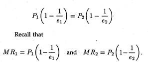
Therefore, the price in market 1, i.e., P₁, differs from price in market 2, P₂ when elasticities in the two markets are unequal. If elasticities were equal, prices would be the same. There would be no price discrimination.

Therefore, if P₁ is greater than P₂, e₁ must be less than e₂. So, it follows that for price discrimi­nation to be effective, elasticities must vary between markets. The elasticity of demand for electricity is low in domestic market due to absence of substi­tutes. Naturally, the price is comparatively high.

Thus, effective price discrimination depends on the difference in the slope of the different demand functions among different markets. The monopolist may now compare profits with and without discrim­ination and choose the optimal alternative.

Diagrammatic Illustration:

Suppose a monop­olist can sell an output in two separate markets, e.g., the CESC which charges two different prices for electricity in two different markets, i.e., a high price in the domestic market form consumers, and a low price in the industrial consumers’ market (i.e., from factories).

And it can effectively prevent the goods from being resold. In Fig. 18.8, we show two graphs. The left-hand graph shows the demand (E>2) and marginal revenue (MR₂) for market 2. In the right- hand graph are shown the D₁ and M R₁ for market;

1. If we add the two demand curves for each price, plotting the points and drawing the line through them, we get the total market demand curve DT- Its corresponding marginal revenue is MRT.

Now, the profit-maximizing output level is one for which MRT is equal to the marginal cost of pro­ducing for both markets, MC. Having chosen the optimum output, profit is maximized by requiring that the MR obtained from selling the last unit in market 1 must just be equal to that earned in market

2. Otherwise there is a chance of increasing profit by shifting units from one market to the other. This requirement is imposed graphically by drawing a dotted line from the intersection of MRT and MC and extending it until it intersects and M R₁ and M R₂.

This happens when the MR obtained from the sixth unit in market 2 is equal to that earned on the third unit in market 1. In market 1, the profit- maximizing price, P₁, is determined by the demand, Dy. Obviously the same commodity is sold at two different prices in the two markets. Thus, the firm is discriminating.

Is Price Discrimination Socially Desirable?

Modern welfare economics examines the impli­cations of charging different persons drastically dif­ferent prices for the same ‘product’ with regard to marginal costs of the seller. Surgeons’ fees are the classic example of this kind of pricing.

What is really important is whether prices produce disparities in ‘real value’ among buyers. Indeed, a good case can be made for the social desirability of many forms of price discrimination (i.e., by cost disparity criteria).

As Dean points out “such discrimination is usually practised by governments and is frequently moti­vated by welfare considerations. Notable examples are subsidized low-cost housing agricultural price supports, unemployment and insurance benefit, and even the progressive income tax. These are all forms of price discrimination that work towards equalising real income.”

Output under Price Discrimination:

The total output of a monopolist with two or more prices can be either larger or smaller than his total output if he would sell at one price. Conceiv­ably, too, a monopolist could have an output equal to the output corresponding to conditions of pure competition.

In practice, demand and cost relations can be such that without discrimination, a particular com­modity or service will not be produced at all. Take the case of India’s sugar industry. If free sale of sugar is prohibited production of sugar will be un­profitable.

Some commodities and services might not be produced at all if sellers were not able, or were not allowed, to practise price discrimination. The standard and simple example is the physician in a small village. Similarly, railroad service on a particular route might depend on the ability of the railroad to charge higher rates to some groups of commuters than to others.

The Algebra of Price Discrimination:

We may how consider a mathematical formu­lation of third-degree price discrimination since it is the most common type. We restrict ourselves to the case of just two submarkets. However, the same analysis may be extended to cover any number of submarkets. Let us assume that demand in market 1 is

P₁ = 98 – 2Q₁

demand in market 2 is

P₂ = 50 – 0.5Q₂

and that the firm has the following linear total cost function (the cost function is assumed to be linear for the sake of simplicity)

C = 1500 + 2Q

where Q = Q₁+ Q₂, or total output. Total profit is

π = Pi + R₂ – C

where R₁(= P₁Q₁) is revenue from submarket 1, and R₂(= P₂Q₂) i^s revenue from submarket 2.

Now we can express profit as a function of Q₁ and Q₂, as follows:

π = (98 – 2Q₁) Q₁-I- (50 – 0.5Q₂)Q₂

– [1500 + 2(Q₁ + Q₂)].

Now by taking the first partial derivatives of profit with respect to Q₁ and Q₂, we can find the profit maximizing quantities, and from them can cal­culate P₁ and P₂.

In the absence of price discrimination, the single price they would charge can be determined as fol­lows. If price discrimination is not practised, P₁ = P₂, and thus (98 – 2Q₁) = (50 – 0.5Q₂), which can be written as (48 – 2Q₁ + 0.5Q₂ = 0).

Adding this constraint to the profit function, we obtain the following Lagrangian function:

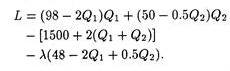
To maximize profit subject to the constraint that prices be equal in the submarkets, we find the fol­lowing three partials of the first order:

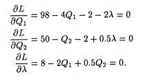
Solving for Q₁ and Q₂, we obtain Q₁ = 33.6 and Q₂ = 38.4. From the market demand equations we obtain the following equalities

P₁ = 98 – 2Q₁ = 98 – 2(33.6) = 30.8

P₂ = 50 – 0.5Q₂ = 50 – 0.5(38.4) = 30.8.

It is now possible to compare the profit in the pure monopoly case with the profit under conditions of price discrimination. In that latter case, profit was found to be 804. With equal prices as in the non-­discriminating case, profit is

Thus, it is clear that this profit is less than that obtained by practising price discrimination.

As a general rule, third-degree price discrimina­tion is supposed to be profitable when the markets can be segregated and when the price-elasticity of demand differs in each market. The higher price will always be charged in the mar­ket with the least elastic demand.

Problem 2:

Suppose two demand functions of a monopolist are:

It is observed that if discrimination is increased, marginal revenues are equal in both markets. By contrast, if prices are equal in both markets, margi­nal renenue in one of the markets is really negative.

In fact, one price must rise and the other must fall under discrimination, but the total profit of the mo­nopolist is higher in the discriminatory case.

Problem 3:

Suppose the two demand curves of the monop­olist are P₁ = 100 – 2_x1 and P₂ = 80 – x₂ and the total cost is C = 20(x₁ + x₂), where P₁, P₂ are prices and x₁, x₂ are the quantities in markets I and II respectively. Determine the equilibrium level of output and prices in both the market.

Solution:

Here

Monopolistic Competition with Product Differentiation:

Monopolistic competition exists when there are many sellers of differentiated products. The demand curve facing the individual competitor is quite elas­tic, but not perfectly so. This important case owes its origin to E. H. Chamberlin.

Monopolistic competition is similar to pure com­petition in that there are a large number of firms sell­ing a product that has been differentiated from that sold by other firms in the industry. That is, although the products sold by monopolistically competitive firms are good substitutes, they are not perfect sub­stitutes.

This, in its turn, implies that the monopolis­tically competitive firm has some control over price, especially in the short-run. Another similar feature of both the purely competitive and monopolistically competitive firm is that both can earn above nor­mal profits in the short-run and normal profits in the long-run.

This follows from the fact that there are no barriers to entry in either of the two market structures. Local retail grocery stores are examples of monopolistic competition.

Chamberlin, in his analysis of monopolistic competition, deals largely with the individual firm’ and does not refer directly to the industry. In fact, it is very difficult, if not impossible, to define an industry in such a situation. Differentiation of prod­uct means that no two firms offer the same product.

Some products may, perhaps, be easily recognized as the same sort of item, but as one get very close to or almost perfect substitute products, one indus­try will coincide with another. Hence, rather than well-defined industries, we get something more like a continuum of products.

Even though the firm under monopolistic com­petition is a very small part of the market as under pure competition, the demand curve for its prod­uct is downward sloping, since customers at large are likely to have different degrees of loyalty to the firms from whom they purchase.

A small reduction in one firm’s price may only attract its competitor’s most valued customers. But if a firm reduces its price drastically, it may be able to attract a large number of customers from its rivals.

As usual, the equilibrium of the firm occurs when marginal cost equals marginal revenue. Again, in the short-run, the firm may or may not earn a profit as under pure competition. There is, no doubt, the possibility of making profits, but there is an equal change of incurring losses.

Under mo­nopolistic competition, there is freedom of entry as under pure competition. Since each firm is small, relatively little capital is required to set up a business and turn out a product which is somewhat different from those already on the market.

The net result is that, as under pure competition, both profits and losses disappear in the long run. The long-term equilibrium of the firm in each market is a tangency solution, i.e., P = AC and no firm can make excess profits, nor it has to incur losses. The average cost curve will be driven toward tangency with the demand curve, and the long-run situation will look like the one shown in Figure 18.9.

The equilibrium point L will be the point of tangency between the average cost curve and the negatively sloping demand curve, D. For at any other output, average total cost will be higher than profit, and so, such an output will involve a loss to the firm.

The average cost curve is normally U-shaped as shown in Figure 18.9, on the ground that both very small and very large outputs are difficult and ex­pensive to produce. As W. J. Baumol put it. “Even economies of large scale apply only up to point, be­yond which administrative costs and diminishing re­turns, because of the presence of scarce (bottleneck) inputs, are generally expected to raise the unit cost of production.”

If this is so, the point of tendency L between the U -shaped average cost curve and the downward sloping demand curve will occur at a point which is to the left of the minimum point M of the AC curve. This is in direct contrast with the equilib­rium of the competitive firm whose long-run posi­tion would have been M.

In pure competition the demand curve of the firm is horizontal and can be tangent to the U-shaped AC curve at the lowest point of the latter. Hence the output of the firm un­der monopolistic competition must be smaller, and its average cost and price higher, than it would be under pure competition.

Thus, from the point of view of the economy as a whole, competitive arrangement appears to be superior to that under monopolistic competition. So from society’s point of view, there is need for some sort of amalgamation of business firms. Figure 18.9 shows that, by becoming larger, firms can reduce their unit costs from what they are at point L.

The implication is that if some of the firms are elimi­nated, the total output will remain unchanged (in­stead of 12 firms producing 500 units each, we can reduce the number of firms to 3, each producing 2,000 units, and so keep the total output at 6,000). But each of the firms will, as a result of its expan­sion, have lower unit costs.

Thus, if the same output is produced at lower unit costs there must be a net overall saving to the community (if unit costs are re­duced from Rs. 8 to Rs. 6, the total cost to the firms producing the 6,000 units in our example, will be re­duced from Rs. 48,000 to Rs. 36,000 — a net gain to society of Rs. 12,000 with no reduction in output).

This result has been called by Chamberlin the excess capacity theorem of monopolistic competition.

Hence, to conclude with Baumol, “only if the elimination of firms results in an important reduc­tion in the variety of products available to the con­sumer, so that a real decrease in consumer choice opportunities occurs, is there any reason for society to “prefer” the product differentiation equilibrium point”, which is L in Figure 18.9.

Duopoly and Oligopoly:

The most prevalent form of market structure in any industry is oligopoly. An oligopolistic in­dustry contains a small number of sizeable com­panies. The product of the rival firms could be both homogeneous or heterogeneous. Duopoly is the minimum form of an oligopoly where there are only two sellers.

In either case, interdependence of decision-making is the characteristic feature of this type of market structure, since actions of any indi­vidual seller have a perceptible influence upon his rivals. If one firm in an oligopolistic industry starts a tremendous advertising campaign or designs a new model of his product which outwit his competitors, he can be fairly sure that this will lead to countermoves by his competitors.

So every business­man in an oligopolistic framework must take into account in his own decision-making the possible re­actions of his rivals, following his decision. Thus, the decision-maker must consider the potential re­actions before changing his price. Here competition takes the form of a battle and advertising and other non-price competition-tricks are the weapons in the individual seller’s arsenal.

However, reactions of rival firms turn out to be very difficult to guess in many situations, as a wide variety of behaviour patterns is possible. There are no generally accepted behavioural assumptions for oligopolists, as there are for perfect competitors and monopolists.

Rivals may decide to get together and cooperate in the pursuit of their objectives to the extent permitted by law, or, at the other ex­treme, they may try to fight each other to elbow out their rivals, or they may choose one relatively large firm (among them) as the leader, and follow his actions.

Even, if they agree to collude, the tacit agreement may last, or it may break down. As a re­sult there are many different solutions for duopolistic and oligopolistic markets, each one being based upon a different set of behaviourial assumptions.

Several models have been developed on different as­sumptions to explain price in such a market. Here we shall discuss the Cournot solution which, though was developed for a duopolistic market, can be generalised for oligopolistic markets too.

The Cournot Duopoly Model:

The model, named after the early-nineteenth- century French economist Augustin Cournot, is the classical solution of duopoly. Here two rival firms are assumed to produce a homogeneous product (e.g., mineral water from two identical wells, as was originally assumed). Also it is assumed that the demand for mineral water is a negatively sloped straight-line function. The demand function looks like

p = F(_q1 + q₂) (1)

where q₁ and q₂ are the levels of the duopolists’ outputs.

Now, the total revenue of each duopolist de­pends upon his own output level, as also on that of his rival

The basic assumption about the behaviour of the sellers is that each duopolist maximises his profit on the assumption that the quantity produced by his rival is invariant with respect to his own quantity decision.

The profit functions are:

π_{1 =} R₁ (q₁, q2) – C₁ (q₁)

π² = R² (q₁,q₂)- C₂ (q₂)

What the above assumption means is this: the first duopolist maximises π₁ with respect to q₁, treat­ing q₂ as a parameter, and the second maximises, π₂ with respect to q₂, treating q₁, as a parameter. Thus

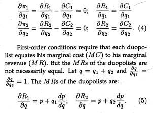
The duopolist with the greater output will have a smaller MR. If either of them increases his output, price will go down, and the total revenues of both will be affected. The rates of change of the total revenues of both will be affected as they depend upon the output levels.

The equilibrium is reached if the values of q₁ and q₂ are such that each duopolist maximises his profit, given the output of the other, and neither de­sires to change his output. The equilibrium values of q₁ and q₂ are obtained by solving the equation sys­tem (4), subject to the satisfaction of second-order conditions:

The solution of the system (4) gives us the re­action functions which express the output of each duopolist as a function of his rival’s output. Thus, We get the following two reaction functions:

q1 = g1 (q₂); q² = g² (q₁) (7)

where q₁ = g₁ (q₂) gives a relationship between and q₂ with the property that for a given value of q₂ the corresponding value of q₂ maximises The second reaction function q₂ =g₂ (q₁) gives the val­ues of π₂which maximises π₂ for a given value of q₁. The solution of the equation system or the reac­tion functions (7), gives us as pair of (equilibrium) values of q₁ and q₂.

Graphical Representation:

The Cournot model may not be represented gra­phically. Cournot assumed that since the firms al­lowed consumers to get their own water and pro­vide their own container, the firms had no produc­tion costs. The marginal cost was zero for each firm. The problem of new entrants was assumed away; entry was totally restricted.

In Cournot’s naive model, the first firm seek­ing to sell its water would treat the market demand as its own. The demand curve is D_m D_m in Figure 18.10, and has a corresponding marginal revenue, MR₁. Since its marginal cost is zero, it would pro­duce where MC — MR₁. The marginal condition is satisfied where MR₁ is equal to zero, which oc­curs at the intersection of MR₁ and the quantity axis.

Thus, the quantity produced is 5. At that quantity, consumers will pay Rs. 5 per unit. The total profit for the firm and the industry is Rs. 25 as shown in Table 18.4. Now firm 2 enters the mar­ket. Because, it is also naive, it assumes that firm 1 intends to produce 5. If it now subtracts 5 from the market demand D_m at every point, it obtains its demand curve, D₂₂, shown on the left as a residual.

It now sets its marginal revenue, M R₂₂, equal to zero. It will maximize profit by producing 2.5 units for a price of Rs. 2.50. If the two firms are located very near to each other and produce a homogeneous product, the first firm will have to sell at Rs. 2.50 also, otherwise it will lose all of the customers.

The two firms jointly will satisfy the market demand of 7.5 at Rs. 2.50 per unit. Their profits under these circumstances are Rs. 18.75, as shown in row 2 of Table 18.4.

The rest of the adjustment process is illustrated in Figure 18.10. The first firm assumes the second will continue to produce an output of 2.5. If we sub­tract 2.5 from the original market demand, D_m, at every point we estimate the demand available to the first firm, i.e., D₃₁. Moreover, setting the marginal revenue equal to zero produces a profit-maximizing output of 3.75.

The reduction in firm 1’s output from 5 to 3.75 reduces the market supply to 6.25, which raises the price to Rs. 3.75. Repeating the process for firm 2 produces D₄₂ and MR₄₂. It is observed that the share of the market going to each firm is mov­ing closer and so are their prices. This process will continue until and unless they are both selling 3.33 units and charging a uniform price of 3.33.

This is, therefore, the Cournot equilibrium. It is to be noted that at equilibrium, the two firms together are not earning as much as the first did by itself, when it had the whole market to itself.

As shown in Ta­ble 18.4, the combined profit of the two firms is Rs. 22.20, whereas firm 1 by itself had a profit of Rs. 25. The prediction is that Cournot’s duopolists provide greater output at a lesser price and earn a smaller profit than a monopolist would with the same mar­ket demand and cost schedules (functions).

One major criticism of the Cournot model has been his behavioral assumption that producers are completely naive. Can they continuously ignore their obvious interdependence?

If the second firm also becomes aware of the in­terdependence, two outcomes are possible. The first is for the two firms to continue to compete but on a more sophisticated basis. The other is for the two firms to collude, that is, to behave like a monopolist.

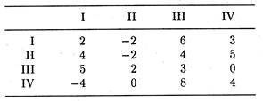
Problem 1:

Suppose there be two firms in an industry and their profits are interdependent, i.e., each one’s profit depends not only on its own output but also on that of its competitor, thus:

π₁ = 24Q1 –Q²₁-2Q²₂-8

π ₂ = 30Q₂ – 3Q²₂ – 2Q₁ – 9.

(i) What will be the of equilibrium outputs and profits if each firm, following the Cournot model, chooses its output to maximize its profit on the as­sumption that there is no reaction from its rival?

(ii) What will the firms’ profits and outputs be if they collude and then set output levels so as to maximize their joint profits?

Solution:

(i) In this case we have to just set the partial derivatives of the profits of the two firms with re­spect to their own outputs as equal to zero. So we get

Surprisingly enough, total profits have risen but the profits of the second firm have fallen under the collusive arrangement. So a reallocation of prof­its may be necessary so that the collusion does not break down.

Problem 2:

Given the following demand and cost functions of two firms I and II, determine their reaction func­tions:

Oligopoly:

Oligopoly means that in an industry, there are few sellers of identical products or differentiated products. The degree to which an industry is dom­inated by a few sellers is measured by the concen­tration ratio. This is the proportion of an industry’s sales that is captured by its few largest firms. For example, India’s automotive tyre industry is domi­nated to a considerable extent by a few large firms.

While there seems to have been a distinct trend over the last two decades towards increased concentra­tion in Indian industries, with large firms getting somewhat larger shares of the market, there is lit­tle tendency for a single producer to eliminate his competitors and emerge as a monopolist from the competitive struggle. Thus, oligopoly is purely a stable form of market organization.

This is largely attributable to the nature of costs. In a number of industries, there are cost advantages, advantages of large scale production. Average cost declines as output rises. When costs actually fall over a considerable range, the development of large firms is encouraged.

But “when costs eventually be­gin to rise while production is still far short of the total quantity sold in the market, they discourage any large firm from growing even larger and devel­oping into a monopoly”. Cost conditions may thus lead to natural oligopoly.

Natural oligopoly occurs when the average costs of individual firms fall over a large enough range, so that a few firms can produce the total quantity sold at the lowest average cost.

A Price Searcher:

The oligopolist is basically a price searcher who lies in the broad area between the polar cases of monopoly and perfect competition. The monopolist has no competitor worth bothering about.

Against, the perfectly competitive firm need not worry be­cause it is only one of many competitors. In contrast, in an oligopoly, the individual firm is very much aware of its few large competitors and necessarily has to worry about their reactions.

So in oligopoly, the firms are interdependent in as far as price setting and decision-making are con­cerned. In other words, each firm is concerned about the reactions of its competitors.

In perfect competition, firms are price-takers. In monopoly, the firm is a price-maker. In oligopoly, the firm is a price-searcher. Although it has some influence over price, this is limited by the possible reactions of its competitors.

Even since Augustin Cournot’s 19th century study of duopoly (two sellers), it has been admitted that the search for an equilibrium price can be quite complex. Oligopoly is one of the least satisfactory areas of economic theory.

Pricing under Oligopoly:

Oligopoly is characterised by administered pri­ces. These are inflexible prices that do not change frequently. The prevalence of mark-up pricing is also widespread.

Oligopoly equilibrium looks like the simple monopoly equilibrium. The point is, in case of a few firms producing homogeneous or identical products, if X’s soap undersells Y’s by even Re. 1 a dozen, A* will get practically all the business. In this case, all firms under oligopoly will recognize their mu­tual interdependence i.e., they will end up charging the same prices.

A price cut will invite retaliation and counter-retaliation and lead to price wars. And each firm will recognize that price cutting begets cancelling out price cutting. Ultimately they realise that they are all in the same boat.

The point that emerges from an analysis of oli­gopoly market organization is simple enough. The typical oligopolist will estimate his demand curve (and market share) by safely assuming that others will charge similar prices. He will also take into account the potential entry of new oligopolists.

So price-cutting is a self-defeating policy. Rather, like a monopolist, the oligopolist will settle for sizable mark-up of price over MC.

Inflexible, administered pricing:

However, oli­gopoly differs from monopoly in one important re­spect. A monopolist usually alters his price as and when his DD or MC curve shifts. On the contrary, oligopoly is featured by more inflexible price quota­tions or administered price.

The model that is dis­cussed here is not designed to deal with oligopolistic price and output determination. Rather, it seeks to explain why, once a price-quantity combination has been decided upon, it will not readily change.

This price inflexibility is basically caused by the fact that ‘rivals may behave in one way when you cut your price, namely, matching your cuts and thwarting your hope for new sales; and they behave in another way when you raise your price above the customary level, namely, holding their prices con­stant in order to pick up some of your customers. The implication is clear.

The oligopolist has little in­centive (and no motive) to change price upward or downward. Rather, the acting firm administers his price in a rigid fashion. It is because each oligopolist learns from his game-theoretic experience that it is easy to agree to a price that is fixed rather than to one that is changing frequently.

The rigid price behaviour can easily be explain­ed in terms of kinked (cornered) demand curve model of oligopoly which purports to show the stability of oligopoly markets.

Prices in a large number of oligopolistic indus­tries seem to have exhibited considerable degree of stability, particularly in their resistance to change in the downward direction. The kinked curve model offers a plausible explanation of such ‘stickiness’ of oligopoly price.

The demand curve for the producer is said to have a kink at the prevailing price because of the asymmetric behaviour of firms in response to varia­tions in prices by the rival firms. It has been argued that competitors follows price decreases but they do not follow price increases by their rival firms.

This is because, if the price is reduced by a firm, its competitors will feel the drain on their customers quickly, and they will be forced to match this price cut. Consequently, the firm which first lowered the price may not be able to increase its sales apprecia­bly.

Figure 18.11 is illustrative of the fact that there is a kink in the demand (average revenue) curve of the oligopolist. Here G is the equilibrium price at which there exists a satisfactory mark-up over costs which is supposed to persist in the long-run.

The reason is not far to seek. If, for instance, the oligopolist cuts his price below G, his rivals will follow suit. Consequently, he moves along the old steep DD curve. In the converse case, when he alone raises his price above the tacit customary price at G, no rival will follow him.

Rather, they will capture a portion of his market share. Even a small increase in price will induce most of his customers to leave him. Prof. Paul Sweezy has pointed out that for price increases, he is on the more elastic dd curve.

This curve simply reflects what he would be able to sell, if he alone changes his price, while all his competitors hold their price constant at G. The corner or kink at G, on the demand (AR) curve gen­erates a vertical discontinuity marked FC, in the MR curve in our diagram.

Here, even shifts of the MC curve in either direction is unable to alter the inherently inflexible oligopoly price. So the solution is stable, in as much as price and quantity at G re­main unchanged.

In the opinion of Prof. Samuelson:

“A ‘cor­nered’ or ‘kinked’ demand curve around an admin­istered level of mark-up price — because price cuts are matched and price increase are not — can help explain the rigidity of oligopoly price compared within both perfect competition and complete mono­poly. Also, this rigidity makes tacit agreement more easily possible”.

The idea of a kinked demand curve was first developed in the 1930’s and it has had con­tinuing appeal as a way of explaining why oligopoly prices are stable, and in particular, why they often remain firm during recessions when demand de­clines.

In the absence of substantial shifts either in demand or cost, price tends to remain at the height of the kink.

Cartel Arrangements:

Oligopololy is also characterized by cartel ar­rangements. Firms often get together and set prices so as to maximize total industry profits. Thus, collu­sive oligopoly resembles monopoly and extracts the maximum amount of profits from customers.

If a formal, overt agreement is made, the group is defined as a Cartel. If a covert, informal agree­ment is reached, firms are said to operate in collu­sion.

If a cartel has absolute control over its members as is true of the OPEC, it can operate like a monop­olist.

To illustrate, consider Figure 18.12 below:

The marginal cost curves of each firm are summed horizontally to derive an industry marginal cost curve. The profit-maximizing output and equi­librium price (P) are determined simultaneously by equating the cartel’s total marginal cost with the in­dustry marginal revenue curve MR_T.

Now each individual firm can easily find its output by equat­ing its marginal cost to the pre-determined industry profit-maximizing marginal revenue level.

Mathematically, this condition will be as fol­lows. The cartel attempts to maximize total industry profit

How profits are shared among firms?

Profits are allocated on the basis of:

(1) Individual output,

(2) Historical market shares,

(3) Production capacity of firms and

(4) Bargaining power of individual firms.

However, cartel arrangements do not last for long due to:

(1) Changing products,

(2) Entry of new firms into the industry and

(3) Disagreement among the members.

But subversion of the cartel by an individual firm can be extremely profitable to that firm. In a monopolized industry the demand curve facing an individual firm is highly elastic, provided it can lower its price without other cartel members learning of this action and retaliating. .

Price Leadership Models:

Any discussion of oligopolistic pricing will be incomplete if we failed to consider the concept of price leadership. Such a situation is characterized by the fact that one firm sets the price and all other firms follow by accepting that price. Two types of price leadership are possible: ‘dominant firm’ model, and the barometric ‘low-cost’ firm model.

(A) Price Leadership by a Dominant Firm:

In this case, a single firm, usually the largest firm in the industry, sets the industry price and al­lows the other smaller firms to sell what they can at that price. Thus, the smaller firms act like per­fect competitors since they have to accept the price as given. In such a situation the effective demand curve for the dominant firm (Dd) is simply the mar­ket demand, less what the small firms will offer for sale at each price.

The supply curves for the follow­ers is their marginal cost curves (they equate P and MC), so that their supply total is S_ƒ= ∑MC for all follower firms. These concepts are illustrated in Figure 18.13 where S_ƒ is the total supply function for the smaller firm and D is the market demand. D_d can be found as follows: D_d = D — S_ƒ. Rd is the dominant firm’s marginal revenue function, and C_d is the dominant firm’s marginal cost function.

The dominant firm will produce the quantity (Qd) for which their marginal revenue and marginal cost are equal and set the price from the Dd demand function at Pd. At this price, the curve S_ƒ shows that the smaller firms will supply (Q_ƒ). The total amount supplied will be Q_d + Q_ƒ, which is not equal to Qt.

There is be likely to only one firm in an oligopo­ly that is generally respected as the best interpreter of changes in costs or in demand conditions, that affect the whole industry. If this is the case, baro­metric firm price-leadership may occur. Other firms may rely on this firm to reflect changes in price that are desirable in the light of changing market condi­tions, and will follow its lead.

(B) Price Leadership by a Low-cost Firm:

This is special case of price leadership by a dom­inant firm. In fact, the dominant firm’s position arises because it has a significant cost advantage over its rivals.

When a particular firm enjoys dis­tinct cost advantage, others will hesitate to compete with the leader because it would apprehend that in the event of a price war, the low-cost leader would easily win out. This fear of retaliation by the low- cost producer forces the rival producers to accept implicitly the dominant firm’s price leadership. This type of behaviour is depicted in Figure 18.14.

Let us assume that there are only two firms in an industry — a typical duopoly situation. A ho­mogeneous product is traded. The- market demand curve is given.

The marginal cost curves of the two firms are MC_A and MC_B, respectively. In Figure 18.14, firm A is the low-cost firm. It will maximize profits by equating its marginal cost with its marginal revenue at point C, producing Q units and charging a price of P. Firm B then has to choose that level of output which miximizes its profit subject to the constraint that its price will be the same as that charged by the low-cost leader.

Thus, firm B’s demand curve corresponds to the line PAD_f. It implies that if firm B sets its price above P, it will lose its cus­tomers to firm A, which is charging a lower price.

Conversely, if it sets its price below P, the low-cost price leader will simply match the price cut as the Sweezy’s model. Thus, there will tend to be some degree of price stability in the low-cost leadership model, as the followers cannot compete on the basis of price because of their higher cost structure.

Even if there is product differentiation between the firms, the general implications of the model are not affected. In this case one would expect to ob­serve a range of prices among the competitive firms, reflecting both the cost differences referred to above, and the demand differences that are a result of the product differentiation.

Typically, if product differ­entiation exists, a historical relationship is likely de­velop in which the leader will tolerate certain price differences among products.

When the price leader adjusts its price by a certain amount, the followers will match their prices accordingly. This has the ef­fect of keeping relative price differentials unchanged (for example, the leader’s price may always be 12% higher).

As we will observed that the common practice of mark-up pricing (i.e., marking up prices by a certain percentage above cost) is one method by which firms in an industry can adjust prices by the same percentage.

Reaction Curves and Oligopolistic Pricing:

We may now examine, at the concluding sta­ge, how an oligopolist may go about setting his price if he gains clear and definite insight about his com­petitors’ reactions to his decisions. ‘ For the sake of simplicity, we restrict ourselves to the two-firm (duopoly) case. Figure 18.15 summarizes this antic­ipated reaction pattern.

Reaction curve R_ƒ R’_ƒ in­cludes all the relevant information about the price reaction of one firm, B, to the pricing decision of its only rival A. For example, point P indicates that if firm A sets the price for its product at OP_a, and if firm B reacts in accordance with the information given by its reaction curve, B would charge price OP_b.

Suppose B stick to this reaction pattern. Now only A’s optimal price decision can be represented. The broken curves in Figure 18.15 represent the in­difference curves of A’s objective function, that is, they are his iso-profit curves if A’s objective is profit- maximization.

Then the highest possible indiffer­ence curve that A can attain (compatible with B’s reaction pattern) is II’. This is tangent to B’s reac­tion curve at point T. To reach this point, A must set his price at OA_m which is indeed his optimal price.

The analysis so far has not given any trouble. But, it is also possible for both firms to play at op­timization. Figure 18.15 contains A’s reaction curve as well, viz., R_aR’_a, which indicates the manner in which B expects A to react to his prices. B, in its turn, may now select an optimum point, say V, on A’s reaction curve, R_aR’_a, and thus he will set his price at OB_m.

But if both A and B choose these “optimal” prices, none will end up on point T or on V. Instead, the resulting price combination is likely to be represented by W, a point which lies on neither reaction curve.

Consequently both firms will be surprised at their earnings — they may either be pleasantly sur­prised (on higher indifference curves than they ex­pected) or they may be actually disappointed. What is more important is that they will both recognise the fact that the reaction curves have become false­hoods, for neither firm is now reacting according to his reaction curve.

As soon as they realise this, they will also come to know that their optimality calcu­lations have gone totally wrong. What was optimal for A so long as B stuck to his reaction curve, need no longer be optimal once B strikes off on his own. Both firms have to start fresh calculations and it is difficult to say where exactly they will ultimately end up.

Decision-Making under Conflict:

The two-firm oligopoly behaviour can be anal­ysed with the aid of game theory developed by Von Neumann and O. Morgensten. Here the outcome of the game depends on the behaviour patterns of the competitors. The game is not one of chance, but one of strategy.

Let us consider a simple duopoly (two firm) sit­uation. The two firms are X and Y. Each has the objective of maximizing its own market share and each has three possible courses of action (different possible combinations of decision variables), for ex­ample, strategy 1 may be high-price and aggressive marketing. We can now construct a pay-off matrix, showing the market share of firm A resulting from different combinations of strategies.

The problem for both A and B is to choose an optimal strategy, i.e., the strategy which maximises market share. Needless to say, the total market share is 100 so that if A gets X per cent, B must get (100 — X) per cent. A knows that B is also try­ing to maximise his market share, so A expects that whichever choice he makes, B will react to minimise the market share of A.

This offers a clue to solving the problem. Since A expects the worst possible re­action from B, A adopts a maximin criterion. To do this A considers what is the worst that could happen for each choice. If he chooses strategy 1, his worst possible market share is 50%, for strategy 2, 55%, and for strategy 3, 45%. Assuming logically that B will do his worst, A would choose strategy 2, where the worst that can happen is a 55% share.

Here B decides in an identical manner, only now a minimax strategy is adopted, since B wishes to minimise the market share of A (and therefore, maximise his own share). He, therefore, selects the least of the column maximum. If he chooses strategy 1, the worst than can happen is that A gets a 55% share.

In this situation, both strategies result in the same expected outcome, a market share for A of 55%. This equilibrium solution is called a saddle- point, and represents a position where neither A nor B would wish to change their decisions.

Such saddle-points, where the row minimum equals the col­umn maximum, need not always exist. Where there is no such point, the optimal choice will be a mix of strategies, where different choices are made in fixed proportions.

The choice of strategy could now be easily sim­plified. However B reacts, for A, choice 2 is al­ways better than choice 3 (results in a higher mar­ket share). Therefore, A will never choose strategy 3, and is said to be dominated by 2. From B’s point of view, strategy 1 is always better than strategy 2, since 1 always results in a lower market share for A (higher share for B).

To calculate the optimum strategy when there is no saddle-point, we may consider the general 2×2 pay-off matrix shown below:

Let the proportion of times A plays strategy I be p₁. Then if p₂ is the proportion of times A plays strategy II, p₂ = 1 — p₁– Similarly, let P₃ and p₄ represent the mixed proportions for B playing I and II, and therefore, p₃ + p₄ = 1.

The problem simply boils down to finding p_1…p₄. To do this we need the concept of the value of a game (V). This is simply the net result of the game when only optimum strategies are adopted. In terms of our notation, the expected value of the game [.E'(V)] is expressed as:

The six simultaneous equations can now be sol­ved for six values P_1…P₄ and λ₁, λ₂, (for obtaining solutions we have added two artificial variables).

If, for instance, (1) is multiplied by b₁, and (2) is multiplied by α₁, we get

This is known as the method of oddments which can simply be stated as follows:

The proportion of times A plays strategy I, is simply the ratio of the absolute value of the other row difference to the absolute value of that row dif­ference. (In terms of our notation, if A plays I and II in the ratio x : y, p₁ = x/(x + y) and p₂ = y/(x + y).

Thus, the proportion of times B plays his strat­egy I is the ratio of the absolute value of the other column difference to the absolute value of that column difference.

Properties of Saddle Points:

The maximin or minimax strategies have a num­ber of important properties. W. J. Baumol has iden­tified the following two properties of such equilib­rium (saddle) points as the most important of all:

Property 1:

This was called by Baumol the protective power of maximin strategies. According to Baumol, a max­imin strategy offers both parties a measure of pro­tection in that A’s maximin strategy gives him the largest share of market which B can be prevented from reducing any further, and B’s minimax strat­egy offers B the lowest share of market for A, which A can be prevented from increasing any further.

A has set up the highest absolutely defensible floor un­der his earnings. Thus, when A plays strategy I, anything B does will either leave his market share at its maximin level, or raise it above that figure. Similarly, B’s use of his minimax strategy places the lowest possible ceiling over A’s pay-off.

By contrast, suppose A had chosen strategy II instead of his maximin strategy I. It is true that if B miscalculates and plays strategy I or IV, this offers A a greater market share than the maximin pay-off, 18. But B then has available a better counterstrategy. He can choose strategy II, which (with A using his strategy II) will confine A to a 5 percent share of market.

In other words, by choosing a strategy other than his maximin strategy, A has left himself un­protected against a countermove by B which gives him, A, less than his maximum-security-level share. Thus, the maximin or minimax strategy is designed to offer both sides maximum protection — it may well be described as the coward’s (or if one prefers, the prudent man’s) strategy.

Property 2:

Where the pay-off matrix possesses saddle point, a maximin strategy is the most advantageous strategy available to the one firm if the other firm chooses a minimax strategy. This explains why the co­incident pay-off matrix entry of the minimax-maxi- min strategy combination, is called an equilibrium or saddle point.

The implication, in Baumol’s own words, is that if one of the two firms plays its min­imax (maximin) strategy, the other is motivated to employ its maximin (minimax) strategy because that is how it can achieve its largest market share. Equi­librium points therefore, possess an element of inner stability in that if one player adopts a strategy con­sistent with the attainment of such a point, the other player is also motivated to do so.”

Example:

Determine the optimal strategies for each player in the following games. Also find out the value of each game to player X:

Hints:

(i) X plays III, Y play II, value of game = 2

(ii) X plays II and III in the proportions ¼._3/4 while y plays I and II in the proportions1/4,3/4. The value of the game = -1/2

This property can be illustrated with the aid of our pay-off matrix. If B plays its minimax strat­egy III, the most which A can obtain is an 18 per­cent share of the market, which he tests by playing his maximin strategy I.

The reason this is so is that since 18% is also B’s minimax pay-off, it must rep­resent the largest figure in column 3 (the worst mar­ket share for B when he plays strategy III). Similarly we see that if A employs his maximin strategy I, the best B can do in response is to employ his maximin strategy III, because any other strategy will give A more than 18 percent of the market.

Property 3:

All equilibrium pairs are minimax-maximin strategies. A pair of strategies a and b (where a is any one of the strategies open to firm A and 6 is one of those open to B) is defined as an equilibrium pair if, whenever firm A choose a, B’s most profitable countermove is 6, and vice versa.

The previous property of minimax strategies, stated in this terminology, is that the minimax-maxi- min strategy combination constitutes an equilibrium pair. In addition, we may now assert that the con­verse of that proposition is also valid, i.e., that any equilibrium pairs of strategies are necessarily minimax-maximin strategies.

Property 4:

Equality of pay-offs of different equilibrium paris. A pay-off table may possess more than one equilibrium pair of strategies. Suppose we call them (a, b) and (a’, b’). However, since by the preceding property, both a and a’ must be maximin strategies for A, they must yield the same security pay-off to A. Similarly b and 6′ must yield the same security value to B.

In other words, any of the four strat­egy combinations (a, b), (a’, b’), (a, b’), (a’, b) must yield the same payoffs. Therefore, if there are sev­eral equilibrium pairs of strategies, and if one of the players picks any such strategy, then the other player can achieve the same degree of protection (minimum pay-off) no matter which of these he chooses.

Property 5:

Maximin strategies may by poor countermoves to non-minimax strategies. The minimax strategy also has an important unattractive feature. Suppose one of the firms is run by managers who are poorly informed or are not very clever, or who simply are willing to take risks, and who, for any of those rea­sons, do not employ a maximin strategy.

Then, the maximin strategy is likely to be unprofitable to the other firm. For example, if B employs strategy I, then it will be strategy III which yields A its highest market share (64 percent) and A’s maximin strat­egy I, will not do as well. In other words, the pru­dent maximin strategy is only guaranteed to be good when playing against another prudent man!