Taxation and Managerial Decisions (With Diagram)

The below mentioned article provides an overview on the Effects of Various Taxes on Managerial Decisions.

Excise Duties and Sales Tax:

An excise duty is imposed on domestic consump­tion spending. It is imposed on a particular commodi­ty or service. It is akin to a sales tax. In India, for in­stance, the Central Government has imposed high rate of excise duty on petroleum products, cigarettes and liquor. Similarly, the State Governments in India impose sales tax on soft drinks, hotel lodging and cinema tickets.

In addition to providing revenue, ex­cise duties or sales taxes are used to achieve certain other socio-economic purposes such as discouraging the consumption of harmful articles like cigarettes or liquor by increasing its retail price.

Similarly excise duties on petroleum products are used as a means of encouraging energy conservation. This approach is common in India and various other countries of Asia and Europe, where excise duties on motor fuel often cause retail prices to be double or triple the whole­sale price of such fuel.

In general, it is the responsibility of the seller to pay a sales tax or an excise duty. Suppose the Cen­tral Government of India imposes an excise duty of 60 paisa per pack of cigarettes. A retailer who sells cigarettes is under the legal obligation to give 60 paisa to the Central Government for every pack sold. Suppose in the current year’s budget the excise duty is increased to Rs. 1.60 per pack.

Now the retailer is left with three options:

(1) He may raise the price of cigarettes fully by the amount of the duty increase;

(2) He may pay the whole amount of the tax himself and maintain the price at the pre-tax level; or

(3) He may increase the price by a portion of the duty increase.

The pricing policy followed by the retailer is of no relevance to the government as long as the retailer continues to pay Rs. 1.60 in excise duty for each pack of cigarettes sold.

It may apparently seem that the retailer will gain by raising the price of cigarettes fully by the amount of additional excise duty. But in certain situations this may not be a rational choice. In fact, rational pricing policy requires a careful consideration of the supply and demand conditions for the product being taxed.

Suppose before the excise duty hike, the retail de­mand and supply schedules for cigarettes are shown in Table 1. The equilibrium quantity is 16 million packs and the equilibrium price is Rs. 10 per pack.

We may now consider the Re. 1 increase in the ex­cise duty from 60 paisa to Rs. 1.60. The prices listed in table 1 show the total amount received by the sell­er. At each price, the retailer has to pay an extra ex­cise duty of Re. 1 more per pack sold. This means that the net amount retained by the seller at any price is Re. 1 less than before. If, for instance, the consumer pay Rs. 10 per pack, the effective price to the retailer is Rs. 9.

This is exactly what he receives after paying the tax to the Government. In other words, a pre-tax price of Rs. 9 is exactly equal to a post-tax price of Rs. 10. But the extent to which sellers will decide to sell cigarettes depends on his total revenue — the to­tal amount of money he receives in the form of sales proceeds before and after the increase in excise duty.

From Table 1 we observe that sellers decide to sup­ply 4 million packs less at each price after the tax in­crease. Thus when price is Rs. 8.50 per pack, the quantity supplied after tax will be 6 million packs instead of 10 mn. packs. The other entries in the last column of the above table are determined in a similar way.

Now to determine the equilibrium price we have to look at columns two and four. The equilibrium quantity, after the tax increase, is 14 million packs and the corresponding price is Rs. 10.50 per pack.

The equilibrium price before the tax increase, was Rs. 10 and the equilibrium quantity 16 million packs. So price rises by 50 paisa per pack due to the tax in­crease. In other words, price rises by less than the amount of the tax because the tax increase is being shared by the buyers and sellers of cigarettes.

The buyers are paying 50 paisa more per pack and sellers are getting 50 paisa less per pack (because they have to surrender an extra 50 paisa per pack to the Govt., in the form of revenue). Obviously the equilibrium quantity (14 million packs per annum) is less than the equilibrium quantity before the tax increase (16 million packs per annum).

The effect of the increase in excise duty on cigar­ettes is illustrated in Fig. 24.1. Here the original sup­ply curve S shifts to the left exactly by the amount of the tax, (i.e., S + T) differs from S by Re. 1 at each level of sales. The new supply curve S+T reflects the in­creased cost to the firm of selling cigarettes.

It shows that less is supplied at any price than before the tax increase. The new equilibrium price of Rs. 10.50 is determined at the point of intersection between the new supply curve and the old demand curve (point F).

In general, an excise duty is not shared equally by buyers and sellers. The actual impact of the duty depends on the elasticity of demand and supply of the commodity being taxed. In Fig 2 we consider four limiting cases. In Figure 2(a) the demand curve is to­tally inelastic.

In this case price rises exactly by the amount of the tax. Consumers now buy the same quan­tity at a higher price. Producers do not pay any tax. This usually happens in case of highly essential com­modities like life-saving drugs or cigarettes (which people consume due to addiction).

Since consumers cannot curtail their consumption of such goods the quantity demanded is totally unresponsive to price change. Thus the prediction is that if the demand for a commodity is completely inelastic the entire tax can be passed on to the consumer by the producer without any difficulty, i.e., almost no loss of sales.

An exactly opposite type of situation is shown in Fig. 2(b). Here demand for the commodity is complete­ly elastic. The supply curve shifts to the left exactly by the amount of the tax. But price paid by the consu­mer does not rise. It is no because consumers can quickly reduce their purchase of the commodity (Q₁ instead of Q₀) to escape the tax.

Thus as a result of the tax increase, the equilibrium quantity decreases, but equilibrium price remains the same because the seller pays all of the tax. The prediction here is that if demand for a commodity is completely elastic at a particular price, any price increase will cause quan­tity demanded to fall to zero. In this case no portion of the tax can be passed on to the buyer in the form of higher price.

Fig. 2(c) shows a situation where the supply curve is totally inelastic. In this case the supply curve does not shift in response to a tax increase. Equilibrium quantity remains the same and the entire tax is paid by the seller. Such a situation was dis­cussed by Henry George in the last century and he made a case for land tax.

The supply of land is total­ly inelastic and the entire return from the land is a surplus (because land is a gift of nature and has therefore no cost of production). Thus a tax may be imposed on land. This will be fully paid by the land­lord. But the supply of land will not fall as a conse­quence. In Fig. 2(c) we observe that the equilibrium quantity remains unchanged and the entire tax is paid by the seller.

Fig. 2(d) shows an exactly opposite type of situa­tion — a situation in which supply is completely elastic. In this case producers can quickly reduce the quantity offered for sale. Thus if they are made to pay even a very small portion of the tax then total revenue will fall. This will cause the quantity of­fered for sale to fall to zero. So consumers will bear the entire burden of the tax if they want to consume the commodity at all.

As a general rule, the effect of the imposition of a sales tax or excise duty on the market price of a com­modity depends on the elasticity of demand and sup­ply.

The following six points may be noted in this context:

1. The more elastic (inelastic) the demand, the lesser (greater) the proportion of the tax to be paid to the consumer.

2. The more elastic (inelastic) the supply, the less­er (greater) the proportion of the tax to be paid by the seller.

3. If demand is completely elastic the consumer pays no tax (i.e., the entire burden is on the seller).

4. If demand is completely inelastic the producers pays no tax (i.e., the entire burden is on the con­sumer).

5. If supply is completely inelastic the consumer pays no tax (i.e., the entire burden is on the seller).

6. If supply is completely elastic the producer pays no tax (i.e., the entire burden is on the con­sumer).

Thus if marketing managers have information about elasticity of demand and supply, they will be able to anticipate the effects of changes in sales tax policies and plan accordingly. However, it is not al­ways possible to make precise estimates of price elasticity of demand and supply. Yet, a rough guess can help managers to make rational pricing deci­sions in response to changes in taxes.

Tax on Profit:

A purely competitive firm cannot make any excess profit in the long run, because it is a price-taker. On the other hand, firms with market power such as monopolists or oligopo­lists may make substantial excess (economic) profit even in the long run. And a portion of the profit may be taxed away by the government.

The following figure shows the effect of the impo­sition of a profit tax on a monopolist. The profit maxi­mising output and price of the monopolist are PQ_m and P_m, respectively. The profit curve is also shown sep­arately. It shows the total profit earned by the mon­opolist at different levels of output. The curve labelled (I), indicates that profit increases with an increase in output up to  Q_m and declines thereafter.

Now suppose a proportional tax of t% is im­posed on profit. The curve, labelled (II), shows after-tax profit at each level of output. We see that the ef­fect of this tax is to reduce total profit by t% at each level of output. However, this tax does not alter the equilibrium level of output.

The firm continues to pro­duce the same level of output as before. The price also remains unchanged at P_m. So the prediction is that in the short run, the entire tax is paid by the firm and its profit gets squeezed. No part of the tax can be passed on to the consumer in the form of higher price.

However, a tax on profits is likely to affect pric­es and output, by reducing the net return on capital employed. This implies that less investment will be made in the industry subject to tax.

Consequently capital will be diverted to other industries and pro­ductive capacity in the taxed industry will increase less rapidly than otherwise (i.e., if the tax had not been imposed). So in the long run, quantity offered for sale will fall and price will rise because of the profit tax.

A lump-sum tax will also have the same effect as shown in Fig. 24.3. The profit-maximizing output lev­el remains unchanged (price also remains unchanged) but every point on the upper curve shifts down by the same amount (i.e., the amount of the tax.)

Even in the long run the lump-sum tax that does not drive a monopolist out of business, has no effect on its price and output, and hence the whole tax is paid by the monopolist.

If, however, the lump-sum tax on profit is so large that, even at the profit-maximizing level of output, profits become negative, the monopolist will close down its operations completely.

The following example will clarify the point.

Example 1:

(a) What output per week would maximise firm X’s profits?

(b) What is the marginal cost of producing 10 units of output?

(c) What would be the effect on output of levying on firm X a lump sum tax of (i) Rs. 40,000, (ii) Rs. 45,000?

(d) Suppose that in a no tax situation the firm were offered Rs. 100,000 to produce 5 units per week for a special customer; that the cost situation is still as specified in the schedule and that any further output can be sold on the market as in­dicated by the revenue schedule. Should the contract be accepted? What, if any, additional output would be sold and at what price?

Solution:

(a) Profits are maximised at the output at which the greatest total profit is made. The profit, when output is 9 units, is Rs. 41,000 and this is the greatest profit made at the given outputs. Hence 9 units is the weekly output which would maxi­mise firm X’s profits.

(b) Marginal cost of producing 10 units of output is the difference in total costs when producing 10 units as compared to producing 9 units. To­tal cost of 10 units = Rs. 91,000 and total cost of 9 units = Rs. 85,000. Hence marginal cost of producing 10 units = Rs. 91,000 – Rs. 85,000 = Rs. 6,000.

(c) (i) A lump sum tax of Rs. 40,000 would add Rs. 40,000 to the total costs at all outputs and the only output at which any profit would be made at existing prices, would be 9 units again. Here profit would be Rs. 1,000 per week, and at all other outputs no profit would be made.

(ii) A lump sum tax of Rs. 45,000 would mean that there will be no output at which total revenue exceeds total costs, i.e., a loss will be made whatever the level of output. If the firm could foresee this situation it would go out of business rather than in­cur this tax. If it could not foresee the situ­ation it would continue its production in the short run, provided it could cover var­iable costs.

(d) To answer this, it is necessary to consider Av­erage Revenue at each output. Then assuming that the first five units of output are sold for Rs. 1, 00,000, the remaining units will be sold at Average Revenue or price, and total revenue can be calculated.

The profit-maximising output is 10 units because here total profit is Rs. 74,000 — greater than that at any other output. He should accept the contract since previously his maximum possible profit was only Rs. 41,000. He would sell 5 further units of output at Rs. 13,000 per unit.

Sales (Revenue) Maximization and Profit Taxes:

We have already referred to W. J. Baumol’s sales maximization hypothesis. It will now be clear that the effect of the imposition of a profit tax on a revenue-maximizing firm will be different from that on a profit-maximizing firm. This point is illustrated in Fig. 24.4. Sales maximization refers to maximization of TR, and TR is maximum (constant) when MR = 0. So the sales maximizing level of out­put is Q₁.

Suppose management sets a profit target of π₀. To maximise sales subject to the profit constraint the firm has to reduce its output from Q₁ to Q₂. Now suppose a proportional profit tax is imposed. Now after-tax profit at Q₂ is less than the target of π₀.

Thus, in order to achieve the sales maximization goal subject to the profit constraint of output π₀ out­put has to be reduced to Q₃, as is indicated by point (on the new profit curve). Price will also increase to P₃ from P₂ (as shown by the points D and E).

Thus the prediction is that unlike a profit- maximising firm, a sales (revenue) maximizing firm subject to a target profit constraint will be forced to reduce output and increase price even in the short run in response to a proportional tax on profit.

Taxes on Inputs (or Factors of Production):

The government often imposes various types of taxes on inputs. Such taxes are based on the usage of certain factors of production such as labour, capital etc. The amount of tax is based on the quantity of certain inputs and in the production process.

The following two types of taxes may now be consid­ered:

(i) A Tax on Labour:

Suppose a firm is in equilibrium at point A in Fig. 24.5 before the imposition of a factor tax. This point corresponds to the least cost combination of inputs. Now suppose a fixed tax of Rs. t is imposed on each unit of labour used by the firm.

The tax will make la­bour relatively expensive and capital relatively cheap (although nothing happens to the absolute price of capital). Now the price of labour will be (w + t) and the slope of the isocost line will be (w + t)/r instead w/r. The isocost line will now rotate close- wise as is indicated by the arrow.

The new iso-cost line C₂C₂ will be tangent to the isoquant at point B. Thus a change in the factor price ratio, due to a tax on wage, leads to a change in the factor proportion.

The production process will now be more capital in­tensive (or less labour intensive) as can be verified by compared points B and A on the same isoquant. In other words, labour will be substituted by capital and the least cost combination of the two inputs will now be K** of capital and L** of labour (instead of K* and L* as was the case before the imposition of the tax).

Thus the prediction is that if technology permits factor substitution (at least in the long run), a tax im­posed on one input will encourage greater usage of the other inputs in the production process. Thus tax­es can be used as instruments of policy.

A tax on in­terest, for instance, may be imposed to encourage the development of labour-intensive industries in a labour-surplus country like India. Likewise a tax may be imposed on energy use to conserver this strategic resources.

(ii) Pollution Taxes:

In most European countries pollution taxes are imposed to prevent environmental decay. A tax on pollution is basically a tax on the use of water and air. By imposing a tax on water and air, these free goods can be converted into economic resources and policy-makers can encourage managers to substitute other inputs in the production process.

Most facto­ries emit smoke and dirt through the chimneys and pollute the environment. If a prohibitive tax (i.e., tax at a very high rate) is imposed on such emissions, firms will find it economically worthwhile to reduce costs by installing pollution control equipment that reduces the amount of emissions.

However, it is diffi­cult in practice to determine the optimal rate of the tax. This is because the assessment of the extra costs or extra benefits of emissions to the producer, has to be highly speculative.

Property Taxes:

Such taxes may be imposed on two types of prop­erties, viz., fixed property and mobile property. If a property is fixed in location, a property tax will be capitalized. The impact of the tax will be totally on the owner of the property (be it land or building). So the market value of the property will be reduced ex­actly by the amount of the tax. When the owner sells the property in future at a reduced price, he will lose.

The situation is different in case of mobile prop­erty like machines, vehicles or other capital equip­ment. If capital does not have a fixed location, it will tend to be transferred to those locations where the tax rate is low. This explains why many business people are transferring their capital from West Ben­gal to Haryana and Maharashtra.

This process of capital transfer from high-tax to low-tax areas will continue until and unless the rates of return are again equalized. However, the rate of return after tax in both areas will be lower than before the tax was imposed.

So the prediction is that a property tax is akin to a tax on certain inputs. As such, by increasing the relative cost of land and capital, the property tax tends to reduce the use of these inputs (provided fac­tor substitution is possible).

If, on the other hand, the amounts of land and capital are fixed, production techniques will remain unchanged. So the only effect of property tax is simply to reduce the market value of the assets.

Tax Preferences:

Taxes no doubt take away portion of the earn­ings of most firms. But it is possible for companies as also corporate managers to reduce tax payments by taking advantage of various tax preferences that are given to various business activities, decisions or conditions.

Three major types of preferential treat­ment given under existing tax laws are discussed here:

(i) Interest Deductions:

Companies acquire finance for investment pur­poses by using a combination of debt and equity fi­nance. However, these two sources of funds are treated differently with respect to tax laws. Interest paid on debt are deductible expense for tax purpos­es. By contrast, the dividends paid to shareholders and the undistributed profit (or funds set aside by the firm as retained earnings) are not deducted in computing tax liability.

The important point to note here is that the prefe­rential treatment of debt under the corporation in­come tax affects the optimal capital structure used to finance investment projects. In short, deductibility of interest payments on debt has the affect of increasing the amount of debt in a firm’s optimal capital struc­ture.

(ii) Investment Tax Credits:

Tax policy is often used by governments to stimu­late investment which is so essential for economic growth. This is why often tax preferences are grant­ed for investment purposes.

One type of concession offered by governments in recent years is investment tax credit (or simply investment allowance). This scheme permits business firms to reduce their corpo­ration income tax liability by some fraction of the firm’s investment spending during the year.

In our discussion of capital budgeting it was argued that firms should invest on those projects which have positive net present value. Let us now consider an investment project that requires an ini­tial outlay of Rs. C and has an economic life of n years. If the rate of discount is r and the after-tax revenue generated by the investment in a given year is (1 – t) R_i, the NPV of the project may be expressed as:

 

 

 

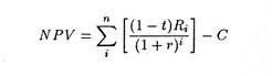
If NPV > 0, the project is considered to be eco­nomically feasible.

Now let us suppose that there is a change in the provisions of the corporation income tax. The tax law allows a 15% tax credit for investment made during the tax year. This credit would allow the firm to deduct 0.15 C from its income tax liability. This means that the actual cost to the firm of the invest­ment would be only 0.85 C.

So NPV of the investment may now be expressed as:

Since the costs are reduced, the NPV increases. Thus the investment tax credit makes profitable in­vestment proposals more profitable. But this is not the whole truth. Investment tax credit serves certain other purposes as well.

For instance, it stimulates in­vestment in projects for which NPV had been nega­tive, but now are profitable because the NPV is posi­tive.

Thirdly, it encourages substitution of other inputs by capital and makes the production process more capital intensive. Since the effective after-tax cost of capital equipment is less than it would be without the tax credit, capital becomes relatively cheap. Hence a firm can achieve cost savings by using more capital and less of other inputs.

(iii) Accelerated Depreciation:

Depreciation expenses are deductible for tax pur­poses. Thus when we make allowance for deprecia­tion, the NPV of an investment is expressed as:

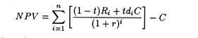
where d_i represents that portion of total cost of the investment which can be depreciated in the i-th year. It is important to note at this stage that the deprecia­tion allowance for any given year increases the NPV of the investment by td_iC/(1+r)ⁱ. It is so because the present value of the firm’s tax liability is reduced by that amount.

If we consider depreciation the NPV may be expressed as:

If C and t remain constant, the NPV increases in­creases with an increases in

depends on the size of the individual d_i. Because the depreciation benefit is discounted to the present, ac­celerated depreciation is attractive to a firm because it allows larger write-offs in the early years of the depreciation period.

This in fact, results in greater NPV than if the rate of depreciation is constant over the economic life of the investment project. Thus if a firm is permitted to depreciate its assets more rapid­ly, otherwise unprofitable projects will be converted into profitable ones, i.e., such projects will now show a positive NPV. The end result will be addi­tional investment in plant, equipment and machinery.