The following points highlight the top seven applications of demand and supply analysis under perfect competition. The applications are: 1. Application on Farm Products 2. Price Control 3. Black Market 4. Consumer’s Surplus and Producers’ Surplus 5. Minimum Wage Legislation 6. Subsidy 7. Taxation.
Application # 1. Application on Farm Products:
There is perfect competition in the market for farm products. Farm products like wheat or rice are usually homogeneous. They are produced by many farmers and each farmer is producing a very small portion of the total supply of a particular farm product, say wheat.
Since total farm product is the sum of the production of many farmers, no individual producer or farmer can affect its market supply. Each producer is a price-taker in the product market. He cannot affect its price and has to accept the prevailing market price. Thus, the market in which the farm products are sold and bought is perfectly competitive.
If the demand and supply forces bring a fall in the price of a farm product, the producer of that particular product shall have to produce more to maintain his income. In fact, there is instability and uncertainty in agriculture. As pointed out by Samuelson, “Farming is an up and down industry.”
ADVERTISEMENTS:
This is because it depends upon the vagaries of nature. A drought or heavy rains may damage the crop and bring misery to the farmer. On the other hand, timely rains and good weather conditions may lead to a bumper crop and bring prosperity to them.
Moreover, agriculture is subject to the law of diminishing returns earlier than in industry because:
(i) Land is limited in supply,
(ii) Agricultural operations are largely dependent on nature, and
ADVERTISEMENTS:
(iii) Economies of large scale production are not available, except on very large farms in countries like America and Australia.
Given these peculiar conditions of farm operations, the prices of farm products are determined by demand and supply.
Demand for Farm Products:
Farm products generally fall under the category of necessary goods. So their demand is less elastic. This means that when the price of a farm product falls, its demand will not rise much and when its price rises, its demand will not fall much. Changes in farm prices do not influence the demand for them because a consumer has to consume these products under all circumstances.
ADVERTISEMENTS:
The consumer spends only a small portion of his income on them. There are no substitutes for these products. The less elastic nature of farm products also implies that when there is a bumper crop, their supply in the market increases. Demand being less elastic, the price of the farm products will fall.
Supply of Farm Products:
The supply of farm products is also less elastic. The less elastic supply is due to the inelasticity of the factors of production at the disposal of the farmers. The cultivable land of producers is fixed and unchangeable. Similarly, farm labour lacks in free mobility.
Moreover, all costs of farm production are fixed and the proportion of variable costs is very insignificant. So whatever quantity a farmer produces, his costs do not change. He will not, therefore, curtail the supply. Rather, he will produce more, in the hope of compensating himself when the price of his product falls. Thus supply increases.
Price Determination:
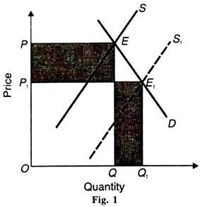
The price of a farm product is determined at a point where its demand and supply curves intersect each other. This is shown in Fig. 1 where D and S are demand and supply curves respectively which are less elastic. Both intersect at point E and determine OP equilibrium price and OQ quantity demanded and supplied.
Suppose the supply of farm product, say rice, increases and the supply curve shifts to the right from S to and the new equilibrium is established at E1 But the demand remains unchanged which brings down the price to OP1 With the fall in price, the supply increases to OQ1 because the producers want to maintain their former levels of income. But the total revenue of the producers falls from OPEQ to OPE1Q1 as measured by shaded rectangles.
Agricultural Price Support:
ADVERTISEMENTS:
The government in developing countries like India generally provides the facility of price support to the farm producers and at the same time, it provides farm products at reasonable prices to consumers. It provides price support so that the prices of farm products do not fall below specified levels.
The government fixes minimum prices:
(i) To protect farmers’ incomes from price fluctuations of farm products, and
(ii) To create buffer stocks to prevent possible future shortages of farm products.
ADVERTISEMENTS:
The specified level of minimum prices is called price floors. It is illegal to undertake any transaction below the price floor.
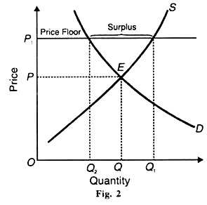
Agricultural price support by the government is illustrated in Fig. 2, where D and S are demand and supply curves respectively. OP is the equilibrium price and OQ the equilibrium quantity. Suppose the government imposes a price floor at OP1 price level above the equilibrium price OP.
At this price floor, the producers are willing to sell OQ1 quantity, while the demand falls to OQ2, resulting in a surplus of Q2Q1 which the government buys as buffer stock. The consumers have to pay higher price OP1 than the equilibrium price OP.
ADVERTISEMENTS:
The surplus is eliminated by the government generally in three ways:
(i) Supply i.e., limiting the acreage of land for the farmers to grow certain agricultural commodities;
(ii) Stimulating demand i.e., new uses for farm products are sought; and
(iii)Purchasing surpluses i.e., certain farm products are bought and stored by the government for future use as “buffer stocks”.
Application # 2. Price Control:
Sometimes the government may think it necessary to interfere in the market process and set maximum (low) price limits for some basic goods. These are known as price ceilings. Producers of such goods cannot charge prices higher than the ceiling prices i.e., the maximum prices fixed by the government.
Price ceilings are generally imposed on many essential consumer goods during war or other critical inflationary periods to prevent them from rising above a certain level.
ADVERTISEMENTS:
In the case of such commodities, the maximum prices fixed by the government are below the equilibrium price. At a price lower than the equilibrium price, the quantity demanded is more than the quantity supplied which leads to the shortage of the commodity. This necessitates the introduction of rationing by the government whereby restriction is imposed on the quantity of a good that a consumer can buy.
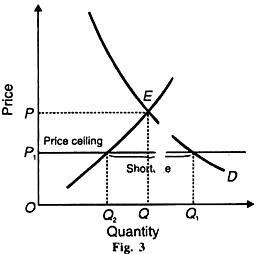
A price ceiling can be illustrated by the normal demand and supply curves. In Fig. 3, D and S are demand and supply curves respectively. They intersect at point E where OP is the equilibrium price and OQ equilibrium quantity.
If the government regards the equilibrium price as too high, it may fix a ceiling price at OP1 .This will result in a shortage of the good equal to Q2 Q1 because OP, price indicates excess demand (O Q1) over OQ2 supply. In this situation, the government may find it necessary to introduce rationing so that the limited goods may be allocated among all the buyers who want them.
Application # 3. Black Market:
Black market of a commodity is the market in which a commodity is sold illegally by the sellers at a price higher than the controlled legal maximum price or ceiling price. It develops on account of excess demand in the market. Some buyers are prepared to pay a higher price for procuring more quantity of the commodity. Sellers are also interested in the black market to sell the products at higher prices and earn more profits.
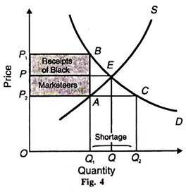
The working of black market is shown in Fig. 4 where D and S are demand and supply curves. They intersect at point E and determine OP market price and OQ market quantity. But the available quantity of the product is OQ1 due to OP2 price ceiling. But the demand is OQ2 and Q2 Q1 is the shortage of the commodity.
Therefore, the buyers are ready to offer OP1 price for procuring more units of the commodity. If the total quantity OQ1 is sold in the black market, the total amount paid by the consumers will be OP1 BQ1 But the receipts of the producers will only be OP2 AQ1 because of the price ceiling.
Thus, the amount OP1 BO1 – OP2 AO1 = P BAP2 will be the extra gain of black marketers shown by the shaded area. However, the entire supply is generally not sold in the black market, because of price laws.
Application # 4. Consumer’s Surplus and Producers’ Surplus:
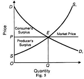
Demand and supply analysis is very helpful in knowing consumer’s surplus and producer’s surplus. Consumer’s surplus is the difference between the a total value that consumer is willing to pay and the payment that they actually makes for the purchase of that product. The total value that a consumer is willing to pay is the area under the demand curve.
On the other hand, what he actually pays is the market price line. Producer’s surplus is the area above the supply curve and below the market price line. It is the difference between the actual amount that a producer receives by selling a given quantity of a commodity and the minimum amount that he expects to receive for its same quantity.
In Fig. 5, DD1 is the demand curve and SS1 is the supply curve. Both intersect at E and determine OP price and PE is the market price line. OQ is the equilibrium quantity. The consumer’s surplus on OQ units of the product is the area EPD and the producer’s surplus on the same units of the product is ESP. The sum of consumer’s and producer’s surplus will be the maximum, when the market structure is perfectly competitive.
Application # 5. Minimum Wage Legislation:
Fixation of minimum wages by the government can also be shown by demand-supply analysis. Fixing minimum wages by the state for sweated trades tends to remove exploitation of labour.
ADVERTISEMENTS:
Minimum wages will so increase the incomes of workers that their consumption expenditures will increase which will, in turn, lead to expansion of the consumer’s goods industries and to the capital goods industries. This will increase employment, output and national income.
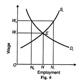
Figure 6 illustrates the effects of fixing the minimum wage above the competitive level. It shows the determination of the equilibrium wage rate OW1 when the demand and supply curves for labour DL and SL respectively intersect at point E.
At this wage rate, ON of labour is employed. Suppose the government fixes a minimum wage of OW2 which is higher than the competitive wage OW1. The increase in the price of labour to OW2 reduces the demand for labour to ON2 But the supply of labour increases to ON1 with the fixation of the higher minimum wage. This excess supply over the demand for labour leads to N2 – N1 unemployment.
Application # 6. Subsidy:
When the government feels that the market price for the farm product is too low for the farmers, it decides to pay them a subsidy. They will receive it in addition to the market price. A subsidy is a government grant given to producers to reduce the price per unit of a product.
ADVERTISEMENTS:
This is to encourage the farmers to produce more which will, in-turn reduce the market prices. The benefits shift from the producers to the buyers which depend on the elasticity of demand and supply.
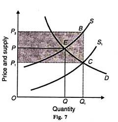
Subsidy shifts the supply curve downward to the right. This is illustrated in Figure 7 where demand and supply curves are D and S respectively. They intersect at point E. OP is the equilibrium price and OQ equilibrium quantity.
The government decides that the farmers should get a price of OP2 for their product. Accordingly if a subsidy equal to BC is granted, the supply curve shifts downward to the right to S1 .The new equilibrium is at C. OP1 is the new equilibrium price and OQ1 the new equilibrium quantity.
Thus, as a result of the subsidy, the price falls to OP1 and the quantity rises to OQ1 .The benefit to consumers is equal to PP1 .They can buy more quantity OQ1 at a lower price OP1 The benefit to producers is equal to P1P2 .The subsidy paid by the government is equal to the sum of the benefits of consumers and producers the shaded area P1P2BC.
Application # 7. Taxation:
The demand and supply analysis is applicable to the problem of incidence of indirect taxation. The incidence of a tax involves the process of transfer from the person on whom the tax is imposed initially to the ultimate taxpayer who bears the money burden of the tax.
The incidence of commodity taxation is shared between the buyers and sellers in the ratio of the elasticity of supply of the taxed commodity to the elasticity of demand for it.
Es/Ed = Incidence on Buyers/Incidence on Sellers
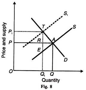
This is explained diagrammatically in Figure 8. Let D be the demand curve and S be the supply curve of the commodity before the tax is levied. OQ quantity of the commodity is sold and bought at QA (=OP) price.
Suppose an excise duty equivalent to ET is imposed on per unit of the commodity, which is collected from the sellers. As a result, the supply curve shifts upward as S1 and the price of the commodity rises to Q1 T (=OP1). But the per-unit increase in price is RT. the difference between the new price (Q1T) and the pre-tax price (QA).
Thus the RT portion of the tax is borne by the buyers and ER portion by the sellers, ET = ER + RT. Given the elasticity of supply, the greater the elasticity of demand for a commodity, the greater will be the incidence of the tax upon the producers and vice versa. Likewise, given the elasticity of demand, the greater the elasticity of supply, the higher will be the incidence of tax upon the buyers, and vice versa.
