Read this article to learn about the Derivation of IS-LM Model in the Short-Run and Long-Run!
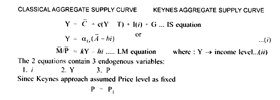
Classical Aggregate Supply Curve and Keynes Aggregate Supply Curve.
In the short run: (Keynes Approach):
In the long run (Classical case):
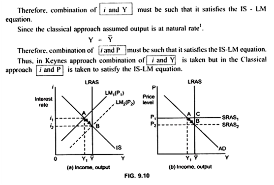
In order to move from the Keynesian equilibrium point (A) which is at less than full employment level, to the Classical equilibrium point (B) which is at full employment level, the price has to fall. Thus, due to low demand (Demand → P1A; Supply → P1C)
P1C > P1A the price falls, and the economy returns back to its natural rate Y .
ADVERTISEMENTS:
In the long run price level will fall till it does not reach the point where aggregate demand equals the aggregate supply. This is at point B. But, decrease in price will affect the Money market. This is because LM curve shows the combination of i and Y where demand for money (L) is equal to supply of money (M).
Therefore, when Price falls with (M) remaining constant, M/P increases. When M/P changes, L will also change. Thus, due to an increase in the real money balances (M/P), the LM curve will shift to the right to LM2(P2) and the interest rate falls from i1 to i2.
As a result the SRAS curve shifts from SRAS1 to SRAS2 and the economy moves back to its natural output, that is at point B.
Thus, in the long run the economy is in equilibrium when
ADVERTISEMENTS:
IS = LM2(P2)
and AD = LRAS = SRAS2
This is attained at point B, at income level Y and at price level P2.
Thus, Long run equilibrium is achieved by a shift in the LM curve.


