Role of AD and AS in the Keynesian Model (With Diagram) | Employment

In this article we will discuss about the role of Aggregate Demand (AD) and Aggregate Supply (AS) in the Keynesian Model, explained with the help of a suitable diagram.

In the Keynesian model an important role is played by aggregate demand, which consists of four components. First, there is household consumption, the main component of aggregate demand. Secondly, there is investment expenditure on producer goods, such as factory buildings and machines. Thirdly, there is government expenditure on goods and services.

Fourthly, there is the balance of exports over imports. In Keynes’ model the level of national output—the amount of prosperity – is determined by the combined forces of aggregate supply and aggregate demand. The classical economists, however, had assumed that aggregate supply conditions alone would determine this.

What happens in the Keynesian model when an increase in government expenditure (on public works such as road construction) takes place? In the Keynesian model when there is productive slack in the economy an increase in aggregate demand leads to a proportionate increase in national output with no change in the general price level, however at a very high level of economic activity with many firms operating close to the limit of their capacity, conditions of aggregate supply would become less elastic.

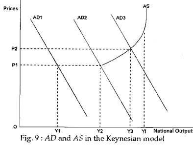
A continuing expansion of aggregate demand would thus lead to rising prices and a smaller gain in output (‘production’). If aggregate de­mand were to expand to a level corresponding to full employ­ment of capacity, aggregate sup­ply would become totally inelastic. The effect would be purely one of rising prices, with no gain at all in prosperity. This point is illustrated in Fig. 9.

In Fig. 9 the aggregate demand curve is seen to be downward sloping. The main reason for this is the real balance effect: as the general price level falls the buying power of money held by households and busi­ness increases, so aggregate spending on goods and services is likely to be higher.

The shape of the aggregate supply curve depends on the assumptions we make. In the Keynesian model it is only partly upward sloping. At low levels of economic activity, when there is a lot of productive ‘slack’ in the economy, aggregate supply is assumed to be horizontal and infinitely ‘elastic’. However as the level of economic activity rises, and firms operate closer to the limit of capacity, aggregate supply becomes increasingly in­elastic.

Assume now that aggregate demand in Fig. 9 increases from AD₁ to a new level AD₂. This leads to a proportionate increase in national output from OY₁ to OY₂, and no change in the general price level, however when aggregate demand increases further, from AD₂ to AD₃, it encounters less elastic conditions of aggregate supply.

The rise in national output is therefore less than for the first increase in demand (AD₁ to AD₂), and there is a rise in the price level, from OP₁ to OP₂. If the expansion of supply were to reach the point OY_f, corresponding to full employment of capacity, aggregate supply would become totally inelastic.

The entire effect of increased aggregate demand would be in higher prices. So, in the Keynesian model, higher consumer spending could lead to a significant increase in national output, with little or no rise in prices — a period of increased prosperity.