Guide to The Basic Keynesian Model (With Diagram)

This article provides Keynesian expertise guide to the model of aggregate demand in an economy.

Introduction:

During 1930s a serious and deep rooted depression, popularly known as worldwide depression, occurred.

During this depression a steep decline in economic activities was experienced.

For instance, unemployment in U.S rose from 3.2 per cent in 1929 to 25.2 per cent in 1933. The GNP fell by 30 per cent and could not be recovered until 1939. In U.K. also the level of unemployment remained around 11 per cent throughout the decade of depression. This caused lot of sufferings to the society and, therefore, gave rise to a debate amongst the economists.

The debate was over the causes of unemployment and policy prescription and its response. British economist J.M. Keynes was a notable participant in the debate during the course of which he developed his revolutionary theory of macroeconomics. His macroeconomics was published in the form of a book in 1936, entitled, ‘The General Theory of Employment, Interest and Money’. This book became the foundation of what is later known as Keynesian Economics.

Keynes pointed out that deficiency in aggregate demand was the cause for high unemployment and falling GNP. According to him fiscal and monetary policies should be so designed as to increase the aggregate demand. The government should spend more on public works during depression.

The other participants in the debate, of course, realized the human sufferings of unemployment but supported the classical economics and believed that unemployment is a temporary phenomenon and downward wage-rigidity was the cause for this. According to Pigou wage cut will make the labourers cheaper and will increase the demand for labourers.

The process of wage cut should continue till the problem of unemployment is solved. Keynes argued that wage cut was no remedy. Why to cut the wage rate? It was deficient aggregate demand which gave rise to the problem of unemployment and then to the problem of wage cut. So aggregate demand should be increased. Moreover, wage cut was also not found as remedy because in United States money wage fell by one third between 1929 and 1933 without slopping the rise in unemployment.

Keynes accepted the significance of equilibrium level of output as an ideal state towards which the economy moves. Contradicting the views of classical model he explained that equilibrium level of output in the economy may not necessarily be at full employment, it can be at less than full employment, at full employment or at overfull employment. According to him equilibrium level of output is one where aggregate demand (AD) is equal to aggregate supply or output (Y) irrespect of the level of employment associated with it.

Y = AD

During depression there is excess capacity in industries therefore, perfectly elastic supply curve of output exists until full employment was assumed at a given state of technology. More and more output can be produced by utilizing additional labourers at a constant price level so long as there are unemployed resources. In such a situation aggregate supply curve would remain horizontals X-axis. When the economy reaches a level of output where all the labourers get jobs is called a state of full-employment or potential level of output (Y_p). If the economy resorts to produce more than the potential level of output the aggregate supply curve would become perfectly inelastic as shown in Fig. 11.1.

Whether the economy actually produces at potential level of output (Y_p) or at more or at less than that, depends on the level or situation of Aggregate Demand (AD) as shown in Fig. 11.1. If the AD curve is AD₁ that intersects the AS curve at E₁ actual level of output (Y₁) would be less than the potential level of output. In case the AD curve is AD₁₁ the actual level of output would be equal to the potential level of output. If the level of AD is raised to AD₁₁₁ then the prices (P) rise to P₁ not the output i.e., only money income rises not real income.

Therefore, it can be stated in the simple Keynesian model that output follows aggregate demand which is contrary to Say’s Law of market that ‘supply creates its own demand’. Keynes entire emphasis was on increasing the aggregate demand. How to increase the AD? This had been a fundamental question behind his general theory. Before, knowing his answer to this question let us know the main assumptions of his model.

Main Assumptions:

(i) There exists deficiency of aggregate demand causing involuntary unemployment. At the prevailing wage rate workers are willing to work but they do not find jobs.

(ii) Perfect competition exists in both factor markets as well as in product markets.

(iii) Only short run behaviour of macro variables has been studied. Population and technology have been assumed to remain constant.

(iv) Depreciation charges have been ignored to make GNP and national income equal to each other. Indirect taxes have also been ignored to avoid discrepancy between the two totals.

(v) In this model all variables are being measured in real terms and not in monetary or nominal terms.

Turning to the question of increasing aggregate demand it is useful to understand its components.

Components of Aggregate Demand:

Keynes emphasized that it was AD which brings changes in the equilibrium level of income and employment. AD comes out of total spending’s comprising of consumption spending’s, domestic private business-investment spending’s and government spending’s on the purchase of goods and services, in a closed economy. In case of an open economy we may add net spending’s on exports and imports to the aggregate demand. These different spending’s have been called as the components of aggregate demand. A brief study of these components is necessary to understand how changes in AD can be brought about.

Consumption Expenditure:

Consumption expenditure constitutes more than 62 per cent of GNP in any economy, hence is the most important component of AD. Keynes believed that purchases of consumer goods and services depend on current income of the households. There can be other factors like size of wealth, future income etc. which may also effect consumption expenditure. But current income has been considered by Keynes as the primary factor to influence consumption expenditure. This fact led to the development of ‘Absolute income hypothesis’ to be studied later on. The relation of consumption expenditure to income is known as consumption function.

Consumption Function:

Consumption f unction has been considered as the most notable contribution of Keynes to economic theory. According to him demand for consumer goods depends upon current disposable income. Every rise or fall in the later leads to direct rise or fall in consumption expenditure. This direct relationship between the two has been termed as consumption function. How much consumption expenditure rises due to a given increase in disposable income?

Keynes answered this question through his ‘Psychological law of consumption’ which states:

“The psychology of the community is such that whenever aggregate income rises consumption also rises but less than the increment in income”.

Increased income gets divided between two parts: one part is devoted to consumption expenditure and another part is saved (Δy = ΔC + ΔS). In this way saving and consumption both rise due to increase in income. Keynes stated that consumption is a stable and rising function of disposable income, i.e., income after excluding net taxes.

This can be written as:

C = ƒ(Yd) or C = ƒ(Y – T) …(1)

where Y_d stands for disposable income

T for net taxes.

According to Keynes, consumption is a linear function of disposable income, i.e., a relationship between the two can be shown by a straight line and an equation given below:

C = a₀ + bY_d; a₀ > 0 1 > b > 0 …(2)

This consumption income relationship as shown by Equation (2) has been graphed in Fig. 11.2, where a₀ is a positive intercept showing some positive consumption expenditure even at zero level of income. It is not influenced by the changes in income but is determined by factors which have not been studied here. The parameter b shows the slope of the consumption function, i.e., the change in consumption expenditure per unit change in disposable income as shown in Fig. 11.2.

Keynes termed this slope relationship as marginal propensity to consume (MPC). Keynes believed that consumption will increase with every increase in disposable income but less than the increase in disposable income (0 < b < 1). In the short run MPC remains stable and constant at every level of income. From the consumption functions shown above we can find the level of consumption expenditure MPC at any level of income a₀ shows the amount of consumption expenditure even at zero level of income, which comes out of past savings (-a₀). At Y₀ entire consumption is financed out of current income.

Average Propensity to Consume and MPCC:

Average propensity to consume (APC) is computed after dividing the total consumption expenditure by the related disposable income.

APC = C/Y_d

On a straight line consumption function (a₀ + bY_d) as shown in Fig. 11.2 (showing constant MPC) APC will be falling with the higher levels of Y_d and increasing with the lower levels of Y_d. APC will be infinity at zero level of Y_d.

It can be computed in the following manner to understand its relation with MPC over a stable consumption functions:

At higher levels of Y_d the product a₀ /Y_d would be decreasing because a₀ is fixed but b (MPC) remains constant. Therefore at higher levels of Y_d APC would be falling and at lower levels of Y_d APC would be rising. It is to note that APC will always be greater than MPC on a straight line consumption function with positive intercept (a₀) as shown in Fig. 11.2. For, APC is a sum of MPC (b) plus a product (a₀ /Y_d ) on such a consumption function. If consumption function originates from zero (a₀ = 0) then MPC = APC. If it originates with negative intercept (a₀ < 0) then MPC > APC. MPC = APC on a consumption function with zero intercept as shown by the Fig. 11.3.

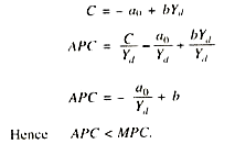
APC would be less than MPC (APC < MPC) on a consump­tion function with negative intercept) (- a₀) as shown by Fig. 11.4. It is theoretically possible that consumption expenditure can be negative (- a₀) at zero level of income. In that case APC < MPC.

 

Marginal Propensity to Save:

Increment in income leads to increase in saving as well as in consumption. The breakeven point shown in Fig. 11.2 occurs at that level of income where saving is neither negative nor positive but is zero as the equidistant line of 45° is intersected here by the consumption function. Further increase in income makes the saving positive. Hence, saving is also a function of income.

We know that national income can be stated:

Y = C + S + T

We know that Y_d = Y – T = C + S

Thus in the Keynesian model a saving income relationship can be established by the equation given below and lower part of Fig. 11.2.

 

Investment:

In Keynesian model investment is crucially important component of aggregate demand. It is a key factor to change the aggregate demand and hence income. Investment here means private business investment only. Importance of investment as a component of aggregate demand rises due to the fact that its another major component, i.e., consumption, is a stable function of income. So it was not possible to change aggregate demand and then income by changing consumption expenditure as it itself depends on income. Keynes invented that investment is an autonomous expenditure determined independent of the level of income.

He found it to be the main cause for the variation and instability in income and employment. The world-wide depression of 1930s was also caused by a fall in investment. For instance, in 1929 the investment was around 16 per cent of the GNP in U.S. which declined to a level of around 2 per cent by 1933.

What determines it becomes an important explanation for knowing the changes in AD and income. Keynes believed that business expectations regarding future profitability of investment or marginal efficiency of capital (MEC) and rate of interest were the main determinants of investment.

Given the stable business expectations or MEC in the short run investment is inversely related to the rate of interest:

l = ƒ(r)

Expectations of future profitability over a new project are formed by investors in spite of the lack of knowledge about consumers’ tastes, aggregate demand, policy of the government etc.

Keynes argued that investors form future expectations on the basis of two factors:

(1) Investors believe that what has happened in recent past will also happen in near future ordinarily.

(2) Investors will judge the future from the behaviour of the group of investors in the economy.

Keynes felt that business expectations were most unstable as they change with new events and information. Their drastic change would change the investment abruptly. Therefore, change in investment is the main cause for bringing change in aggregate demand and the resultant change in the level of income.

Government Expenditure:

Government expenditure is a third major component of AD. Like investment expenditure government expenditure is also known as autonomous expenditure. It is autonomous because it is primarily determined by policy-makers and not by income, hence, is also an exogenous variable.

Though changes in income make changes in tax collections at a given rate of tax and tax collection is the source of government expenditure over purchase of goods and services. In this way one can say that government expenditure is also endogenously determined by income. But it is not true because tax rates are determined by policy makers. Hence, Government expenditure on the purchase of goods and services is autonomous and not at all induced by income in our analysis here.

Determination of Equilibrium Level of Income:

In Keynesian model equilibrium level of income or output is one where total output (GNP) is equal to aggregate demand.

It can be expressed by the equation:

Y = AD

The proceeding section shows that the components of aggregate demand are consumption expenditure (C), Intended investment expenditure (i) and the government expenditure on the purchase of goods and services (G).

At equilibrium level of output, therefore condition (i) can be written as:

Y = AD = C + i + G

Since Y is total output consisting of consumption goods (C), investment goods like machinery, tools and plants etc. also known as real investment (i_r) and the goods and services for government purchase (G), it can he expressed as:

Y = C + i_r+ G

Combining equations (ii) and (iii)

C + i_r+ G = C + i + G

Cancelling C and G from both sides we have

i_r = i

meaning thereby, equilibrium level of output which is an endogenous variable can take place only at a level where intended investment (i) is equal to real investment (i_r).

If (i), intended investment is greater than i_r, real investment (I > i_r) then AD would be greater than AS or total output. The businessmen will meet this extra demand by declining their inventories which they maintain of a size considered ideal. This involuntary fall in their inventory size will induce them to place fresh orders to the producers and, hence, output and employment will rise. Contrary to it, if i < i_r the size of their inventories will expand involuntarily.

To maintain their voluntary level of inventory, which is considered to be ideal, the businessmen reduce their orders to the producers for fresh purchase of goods. As a result total output contracts, hence, a fall in output and employment takes place. Therefore, equilibrium level of output can be one where intended investment is equal to real investment.

Another condition for equilibrium relates to leakages (S + T) and injections (i + G) shown in the circular flow of income. Equilibrium level of output (or a constant flow of income) is possible only if leakages are equal to injections.

Hence, this condition can be expressed as:

S + T = i + g

If the two sides are not equal a change in output is bound to occur.

So there can be three condition for equilibrium level of income:

Y = AD = C + i + G …… (i)

r = i ……. (ii)

S + T = i + G ….. (iii)

Determination of equilibrium level of income satisfying above conditions can be shown with the help of Fig. 11.5:

The income level (Y_d) is being measured along horizontal axis and the aggregate demand, along with its components, are being measured along vertical axis. Every point of 45° line shows equal distance from both vertical and horizontal axis. Autonomous expenditure like investment and government expenditure do not depend on income, at least directly. The C + i + G schedule, therefore, lies above the consumption function by a constant amount. The fact that (i + G) does not depend on income is also reflected by the i + G line being horizontal to X-axis. Saving plus taxes (S+7) line slopes upward because saving and taxes vary positively with income.

Equilibrium level of income takes place at Y where the aggregate demand curve (C + i + G) intersects the line of 45^o. Here (S + T) is equal to (i + G). At point Y aggregate demand (C + i + G) is also equal to output (Y) showing equilibrium level of income. If the actual level of output is below Y, say, at Y₁ in Fig. 11.5, the AD (C + i + G) would be greater than output (C + i_r + G) by AB.

Intended investment (i) would be greater than the real investment (i_r), (i > i_r). In such a situation inventory will decline below the desired level. Output has to be increased to recover inventory so income would start rising through multiplier to reach Y, the equilibrium level of income. If level of output is at Y₁₁ then aggregate demand (C + i + G) falls short of output or supply by KL and i < i_r. Then the level of output will decline through, multiplier. For, inventory level goes up above the desired level, ultimately, the equilibrium level of income (y) is attained by the economy where C + i + G = C + i_r + G, or i = i_r.

Change in Equilibrium Level of Income:

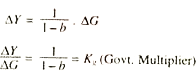
Equilibrium level of income can change either due to change in the value of multiplier or due to change in expenditure, because, equilibrium level of income is determined in any time by the two, i.e., the value of multiplier and the amount of expenditure. We know that

Thus, it is true to say that Y depends on the value of autonomous multiplier and autonomous expenditure increased at any time. Both are autonomous as they are independent of income. Therefore, to change y either the value of multiplier or autonomous expenditure or both units must change.

But the value of multiplier remains constant because MPC (b) is stable in the short run, which determines its value. Hence, the equilibrium level of income can change only by changing the autonomous expenditure. In other words, as per equation (iv), to change Y either the investment expenditure (i) or government expenditure on purchase of goods and services (G) or tax collection (T) must change.

Keynesian Model without Government or Change in Equilibrium Level of Income due to Change in Investment:

In a situation where only private business investment changes and government expenditure (G) and taxes (T) i.e., net taxes remain constant then how much change in equilibrium level of income occurs? This is a most simplified model where it has been assumed that either the Government is totally inactive or there is no government. No international transactions are made. GNP, NNP and disposable income have been assumed to be the same.

In such a world income will be:

Equation (v) shows that for any value of i there is a corresponding value of Y in a static model like this. Suppose, i is increased and its increment is shown as Δi.

Then total investment expenditure would be i + Δi corresponding to a new equilibrium level of income (Y + ΔY):

It is clear that the value of K depends on b. Change in income (ΔY) would occur in accordance with the value of K and Δi.

It raises two questions:

(i) Why does income increase by a multiple increase in i?

(ii) Why does income rise exactly equal to 1/(1 – b) Δi and not more or less than this?

Consequent upon the increase in investment expenditure, say, of Rs. 100, the income in the economy would rise instantaneously by Rs. 100 in the form of wages, interest, rent and profit of the owners of various factors of production. This is a direct effect on demand and income.

This increased income will stimulate further increase in demand for consumer goods which is known as income induced demand. People will spend on consumption a part of this increased income of Rs. 100 according to their MPC (b). Suppose MPC = .8. In that case only Rs. 80 would be spent on the purchase of consumer goods (naturally Rs. 20 will be added to saving) raising income of the sellers of these consumer goods, as the spending by one is the income of the other. This process will continue and the income will, ultimately, rise by more than the autonomous rise in investment due to induced increases in consumer demand as income rises. Now, second question as to why increase in income is just equal to 1/1-b Δi?

This is so because so long as demand exceeds supply income continues to rise. As and when the two become equal the income finds equilibrium level. At equilibrium level of income.

S + T = i + G

Since T and G are absent or constant here then i = S. To maintain equilibrium level of income, any increase in i must be accompanied by an equivalent increase in S. such that:

Δi = ΔS

To restore equilibrium income must rise enough or to a level that may generate new savings equal to the new investment. This is shown graphically where Y is measured horizontally and C and i vertically in the Fig. 11.6.

A fixed amount of i determined exogenously is added to the consumption function (a₀ + bY) which form the aggregate demand establishing equilibrium at E₀ determining Y₀ level of equilibrium income. Increase in investment shifts the aggregate demand function to (C + i + i) which intersects the 45° line at E₁ establishing new equilibrium level of income at Y₁. In the process saving rises with the increase in income along the saving function. Income continues to rise until ΔS = Δi which is possible only at Y1. Income has rise more than the increase in investment and exactly equal to (1/1-b.Δi)

The effect on equilibrium level by income of change in rest two of the autonomous expenditures (G and T) can be calculated from equation (iv).

Keynesian Model with Government: Change in Income due to Change in Government Expenditure:

Here, it has been assumed that government expenditure (G) on the purchase of goods and services rises and i and T remain constant. Increase in G will have the same effect on demand as the increase in i, as we have seen in the preceding section. In both the cases initial increase in income is equal to increase in spending (i or G) and income induced increase in demand for consumer goods (depending on b) is also the same. Hence, the multiplier process is the same.

Therefore :

The increase in equilibrium level of income as a result of increase in G can be shown graphically.

The Fig. 11.7 shows that the AD curve C + I + G shifts to C + I + G₁ as a result of an increase in government expenditure on goods and services. Consequently Y₁ equilibrium level of income settles down where (I + G) is again equal to s + T as they were at Y₀ level of income. Government multiplier ΔY/ΔG is the same as was the investment multiplier(ΔY/Δi)

Change in Income due to Change in Taxes ( T):

Taxes (T) means net taxes i.e.. transfer expenditure (Expenditure on pension, unemployment allowance etc.) has been deducted from total tax collection by the government. Equation (iv)shows that the effect of an increase in taxes is in the opposite direction from those of either an increase in government spending or investment.

In the equation keeping other things constant increase in T would change income: ΔY =1/1-b (-b ΔT) i.e., increase in taxes (T) would bring a multiplied decline in the level of income. Why so? Increase in T will lower the disposable income (Y- T). This will shift the consumption function downward by (- b ΔT), hence, the aggregate demand function will also shift downward according reducing the equilibrium level of Y. Change in income can be calculated with the help of tax multiplier and the given change in the amount of tax collections (T).

Increased T (ΔT) will shift the consumption functions downward by (- b ΔT) and accordingly the aggregate demand function to (C + i + G)₁ reducing the equilibrium level of income from Y₀ to Y₁ .This is a multiplied fall in Y determined by [ 1/1-b-bΔT)

 

Keynesian Model in an Open Economy:

Due to imports (M) and exports (X) demand for commodities in the economy changes by net exports (X – M). Demand for our (X) is an addition to aggregate demand and our demand for imports (M) is a decline in the demand for our commodities. The income which could have been spent in demanding domestic goods is being spent in demanding foreign goods. Our imports increase the aggregate demand for foreign countries. Net effect on demand (AD) can be known by deducting the amount of imports from the amount of exports (X – M).

Another point to be noted is that demand for exports is independent of the income in the domestic country. Demand for our exports depends on the income of foreigners hence is exogenously determined whereas demand for our imports is a rising function of the income level in our country, hence, it is endogenous variable. This can be graphed as

Our (X) in the Fig. 11.9 are fixed at X₀ whatever be the level of income in our country. Imports are a rising function of income shown by the linear function, M = M₀ + mY 0 < m < 1, where m₀ is positive intercept showing minimum amount of imports even when income level falls to zero, m is the marginal propensity to import, MPI (m) of the import function. At Y11 level of income there is net addition to our AD because X > M, at Y₀ the imports are equal to exports (M = X) showing no effect on AD, and at income beyond Y₀, say at Y₁ the AD will decline due to foreign trade by the difference (X < M).

Change in income-due to imports and exports can be computed with the help of our old equation.

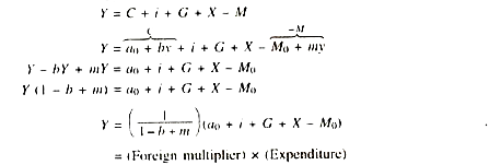
The value of multiplier in a closed economy 1/(1 – b) would be greater than that of an open economy 1/(1 – b + m). Students can examine this by assigning different values to b and m.

From equation (vii) multiplier effects of changes in (X – M) can be computed:

ΔY/ΔX = (1/1-b+m)

Determination of equilibrium level of Y can be graphed in Fig. 11.10.

Due to introduction of exports and imports income the aggregate demand function shift to C + i + G + X- M raising equilibrium level of income from Y₀ to Y₁. The net increase in demand (X – M) goes on falling at higher levels of income due to rise in imports (exports remaining constant).