Linking Variables between Interest Rate and Income

Let us make an in-depth study of the linking variables between interest rate and income.

Introduction:

The interest rate and income are linking variables transmitting changes from the monetary sector to the goods sector and from the goods sector to the money sector. We now examine this relationship in more detail and analyse the concept of general equilibrium in the whole economy, consisting of the goods and money sectors.

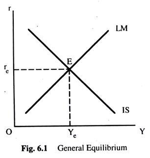
Fig. 6.1 is a summary of equilibrium in the two sectors. The IS and LM curves represent the conditions that have to be satisfied in order for the goods and money sectors, respectively, to be in equilibrium. Now our task is to determine how these markets are brought into simultaneous equilibrium. For simultaneous equilibrium, interest rates and income levels have to be such that both goods market and money market are in equilibrium.

That condition is satisfied at the point E in Fig. 6.1 which is the point of general equilibrium. This occurs at one combination of real income and the interest rate r_e and Y_e and with this combination of income and interest rate there is no tendency for anything to change; individuals are in equilibrium in their allocation of wealth among different assets, and in their allocation of output among different uses.

Even though we are not concerned with the problem of economic dynamics, it is nevertheless important to understand the economic forces generated in this equilibrium, which tend to bring the system back to equilibrium.

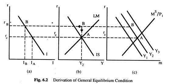
Fig. 6.2(b) represents the equilibrium conditions for the goods and money sectors. Fig. 6.2(c) shows the money sector from which the LM curve in Fig.6.2(b) is derived and Fig 6.2(a) shows the desired investment schedule which together with the consumption function (not shown here) was used to derive the IS curve in Fig 6.2(b).

Point A shows the combination of real income (Y₂) and interest rate (r_e) , respectively, which represents general equilibrium for the economy. At point A in the money sector, the quantity of money demanded shown by the demand curve Y₂ is equal to the quantity of money supplied. At the interest rate r_e, desired investment is equal to I_A – this is shown in Fig. 6.2(a). As point A is on the IS curve, we know that saving generated by a real income of Y₂ is equal to I_A, because every point on the IS curve represents a situation in which saving is equal to desired investment.

Let us consider point B in Fig. 6.2(b) which shows the combination of real income and interest rate Y₂ and r_B, respectively. We want to know what forces will be generated when the economy found itself in the situation represented by point B, and how these forces will work to bring the economy back to equilibrium. We know that at point B neither the goods nor the money sector is in equilibrium, because point B, is off both the IS and LM curves. Thus, something will have to change in both sectors.

In the money sector 6.2(c), we can see that at the combination of income and interest rate represented by point B, the quantity of money demanded is less than the quantity of money supplied. Individuals will try to re-allocate their wealth from money to bonds, thus pushing interest rate down. The arrow pointing down at B represents this tendency.

At panel 6.2(a), we see that at the interest rate r_B, desired investment is I_B. However, at real income Y₂, saving is equal to I_A, because we assume that S is a function of real income only; thus at point B, S > I_B. Hence in the goods sector, point B represents a situation in which AD < Y. Given our present assumption about the effects of a disequilibrium in the goods sector, S > (desired) I will tend to reduce output (real income).

The arrow pointing to the left at B represents this tendency. (According to our assumptions about the goods sector disequilibrium, this only affects output, not the price level and as such it does not affect the LM curve).

The initial forces generated in disequilibrium have further repercussions on the whole economic system. The fall in the interest rate generated by excess supply of money will affect desired I =f(r). The fall in real income F generated by S > I (desired) in the goods sector will affect the demand for money, which is a function of real Y only. As the interest rate falls, desired I rises, reducing S > I (desired). As real Y falls, the demand for money and the interest rate fall, strengthening the effects mentioned above. All of this will continue until point A is reached — equilibrium point, in Fig. 6.2.

Disequilibrium and Dynamics in the Goods and Money Market:

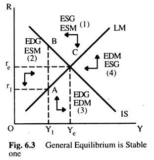
Equilibrium is said to be a stable one when economic forces tend to push the market towards it. Fig. 6.3 shows that the general equilibrium described here is indeed a stable one. To show this, we consider all the points to the left of the IS curve, like point A where interest rate r₁ and the level of Y₁ are too low for equilibrium to be achieved in the real sector. This means that the total value of output is less than the demand.

In this situ­ation, businesses find their inven­tories run down involuntarily and so act to increase output which pushes up Y. For all points to the left of the IS curve, there is an excess demand for goods and thus there is pressure on income to rise. Similarly, tor all points to the right of the IS curve, there is excess supply of goods and there is pressure on Y to fall.

Now we consider points above the LM curve, like point B. At this point, with the level of Y, OY₁, the interest rate is too high for money market equilibrium to be achieved. This means that the supply of money exceeds the demand for money and so downward pressure is exerted on the interest rate. This is true for all points above the LM curve, as shown in Fig. 6.3 and it is also true that upward pressure will be exerted on interest rates at all points below the LM curve as there is excess demand for money.

The direction of the pressure being exerted on incomes and interest rates in the four quadrants are indicated by arrows in Fig. 6.3. At any disequilibrium point, such as C, economic forces will be pushing the market towards the general equilibrium position.

Shifting the IS and LM Curves:

Having analysed equilibrium in the two sectors, it is useful to examine how changes in behaviour will affect the two variables in which we are interested at present — real income and interest rate. There are four behavioural functions that determine equilibrium in the two sectors – the investment function and consumption function and the supply of money function and the demand for money function.

These functions were used to derive the IS and the LM curves and thus the behaviour represented by these functions is held constant along the IS and LM curves. A change is behaviour can be represented by a shift in these functions. Such shifts will result in the shift of the IS or LM curves, or, both.

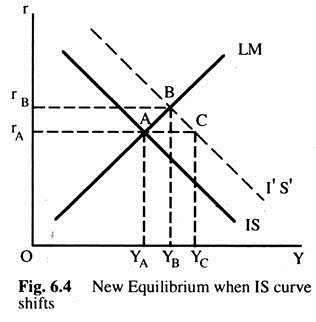
Let us start from a situation of general equilibrium as shown by point A in Fig. 6.4. This is an equilibrium for that set of behavioural functions which underlies the derivation of the IS and LM curves intersecting at A. We now assume that for some reason, desired expenditures increase. For example, suppose there is an increase in desired investment at all interest rates (a shift in the investment function) or a rise in desired consumption at all income levels (a shift in the consumption function). These changes can be represented by a shift of the IS curve from IS to I’S’.

Now the economy is no longer in equilibrium at A because the goods sector now represented by I’S’ is no longer in equilibrium. However, the money sector is still in equilibrium as there is no change in the behaviour of the functions which affect money sector. We know that with the new IS curve, point A represents a situation in which desired expenditures are greater than total output (or I > S ). This will lead to an increase in Y.

As real Y rises, point A no longer represents equilibrium in the money sector either, because the increase in real Y affects the quantity of money demanded and thus equilibrium in the money sector will also change, though has been no behavioural change in the money sector (and hence the LM curve does not shift; there is a movement along the curve). The rise in the interest rate will’ have effects on desired I and on real Y.

This process will continue until a new equilibrium is reached at B with interest rate at r_B and real income at Y_B. At B, both the money and goods sectors are in equilibrium. It may be pointed out here that if the shift in desired expenditures or AD had not affected the interest rate, real income would have changed from Y_A to Y_c, which is equal to the initial change ‘in AD x the multiplier. This would be true if the LM curve is horizontal. Real Y only rises to Y_B because some of the initial increase in AD is offset by the effect of the rise in the interest rate on desired I, called the ‘crowding-out effect’.

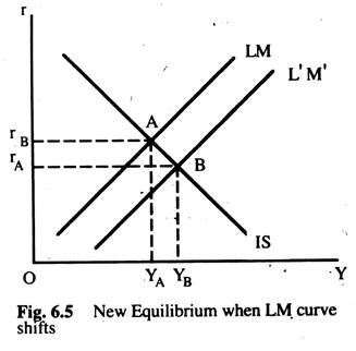
A shift of the LM curve can occur because of a change in the demand for money or in the supply of money. An increase in the supply of money or a decrease in the demand for money can be represented by a shift of the LM curve to the right. To examine the effect of such changes, let us again start from a position of equilibrium at point A in Fig. 6.5. Assume there is an increase in the supply of money brought about by an open-market operation by the monetary authority. With the new money supply, equilibrium in the money sector can be represented by L’M’ curve in Fig. 6.5.

At A, the goods sector is still in equi­librium, since nothing has hap­pened to change the IS curve. However at A, the quantity of money supplied is greater than the quantity of money demanded as the situation in the money sector represented by the L’M’ curve. Individuals will be attempting to reallocate their wealth from money into bonds, thus driving the interest down.

The fall in interest rate also affects the goods sector via its effect on desired I; thus point A will not remain an equilibrium point for the goods sector either. The changes in the goods sector thus generated will have repercussions on the money sector. The process will continue until a new equilibrium is reached at point B, at which both sectors are in equilibrium again.

The above discussion shows how changes in one sector of the economy are transmitted to the other sectors, and how the final equilibrium of the whole system is reached. It is obvious that changes occurring in one sector can only be transmitted to another sector if there exist variables linking the two sectors, and if these changes affect these linking variables.

In our model, the linking variables are the interest rate and real Y. The interest rate is an effective linking variable, transmitting changes of behaviour occurring in the money sector to the goods sector, because the change in the money sector had an effect on the interest rate and the interest rate enters in the goods sector through investment decisions.

Real Y is an effective linking variable, transmitting changes of behaviour in the goods sector to the money sector, because changes of behaviour in the goods sector has an effect on real income Y and real Y enters into decision in the money sector through changes in the demand for money.

To get a better idea about these linking variables, we examine the following cases:

i. The Perfectly Elastic Demand for Money or the Liquidity Trap:

We have already seen the interest rate as a measure of the alternative cost of holding wealth in the form of money rather than in the form of other assets and thus, as a measure of the cost of acquiring the services yielded by money. When the interest rate is zero, the cost of acquiring services provided by money is zero and people will be willing to hold all their wealth in the form of money rather than other assets.

It is possible that even when the interest rate is positive, the expected cost of holding wealth in the form of money is zero. We have already seen that one of the costs of holding bonds is the risk of capital loss arising from a change in the interest rate. When the interest rate rises, there would be a fall in the capital value of bonds; the expected return from holding a bond is equal to the interest yield minus the expected capital toss. If these two are equal, the expected final return is still zero, even though the interest yield is positive.

Assume for the moment that the interest rate is considered to be normal, say, r_n. If the interest rate falls below r_n , individuals expect it to return to r_n and thus they expect to suffer a capital loss if they hold bonds. Let r_L < r_n be the interest rate which would cause capital loss if the interest rate rises from r, to the expected rate r_n which exactly offsets the return represented by r_L.

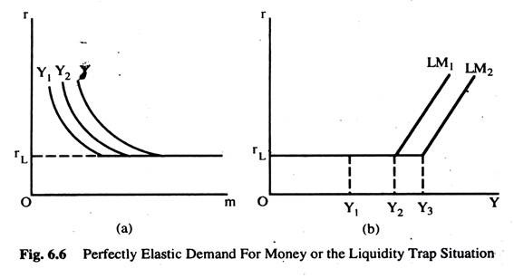
In this case, at the interest rate r_L, the expected return from holding a bond is zero. At the interest rate above r_L, it is positive, and at an interest rate below r_L, it is negative. This case is represented by a demand curve for money which becomes perfectly elastic at the interest rate r_L in Fig. 6.6.

Fig. 6.6 (a) shows 3 demand curves for money for three different incomes, where Y₁ < Y₂ < Y₃, having the property that at the interest rate r_L they become perfectly elastic — at this interest rate people are willing to hold all their wealth in the form of money. M^s1 and M^s2 are two different supply curves of money. In Fig. 6.6 (b), the LM curves are derived to represent this situation. They are perfectly elastic at the interest rate r_L for incomes up to Y₂ for LM₁ and up to Y₃ for LM₂.

The increase in money supply from M^s1 to M^S2 only affects the elastic part of the LM curve, because an increase in the supply of money along the perfectly elastic part of the demand curve for money has no effect on the interest rate. Individuals are willing to hold more money, rather than bonds at r_L, where the cost of holding money is zero and individuals are indifferent between money and bonds.

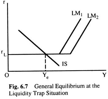
Fig. 6.7 represents a general equilibrium situation for a goods sector represented by IS curve and a money sector exhibiting the properties above, represented by LM, with equilibrium for both sectors on the horizontal part of the LM curve at Y_e and r_L, respectively. Assume there is an increase in the supply of money shown by a shift of the LM curve from LM₁ to LM₂. This has no effect on the equilibrium value of real Y or the interest rate because the part of the LM curve affected by this change is not relevant to the determination of equilibrium.

ii. The Supply of Money is Perfectly Elastic:

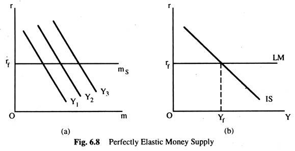
This happens when the monetary authority decides to fix the interest rate at some given level. To do this, they will have to supply whatever quantity of money is demanded at that rate, otherwise the interest rate would be affected by the excess demand or supply of money and would not be maintained at the desired level. This is shown in Fig. 6.8(a) which shows a supply curve that is perfectly elastic at the interest rate r_f and three demand curves for three incomes. In Fig. 6.8(b), we derive the LM curve for this situation. It is perfectly elastic at the interest rate r_f. We can see that any changes in the demand for money (or price level) will have no effect on the LM curve.

If we draw the IS curve on the LM curve of Fig. 6.8(b), we have the same general equilibrium situation as the one in Fig. 6.7. Again changes in the demand for money (or price level) will have no effect on equilibrium Y or interest rate. This is the situation which Keynes experienced and thus, he advocated fiscal policy as an effective instrument for influencing the economy.

iii. The Perfectly Inelastic Investment Function:

The IS curve represents all the combinations of income and interest rate at which AD = Total Output. Both the interest rate and real income are relevant here because we assume that both these variables affect decisions about AD; the interest rate affects desired investment and real income affects desired consumption.

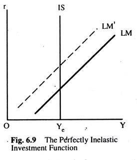
If we now drop the assumption that desired investment depends on the interest rate, real Y becomes the only variable that affects AD, and the IS curve in such a situation will be perfectly inelastic. Fig. 6.9 shows such an IS curve with two LM curves representing two different conditions in the money sector (two different supply functions).

With both LM curves, general equilibrium in the two sectors occurs at the same real income but at different interest rates. Thus any changes in the money sector (shifts in the LM curve) only affect the interest rate, but leave real Y unchanged. However, changes in the goods sector (shift of the IS) affect both real Y and the interest rate.

iv. The Real Balance Effect:

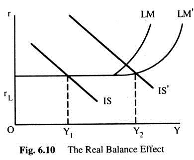
The Neo-Classical economists, mainly Prof. Pigou, produced an argument against the Keynesian liquidity trap case in the shape of real balance effect. According to this, with a constant nominal money supply, a general deflation of wages and prices tend to increase the real value of people’s holdings of money above their desired levels.

Consequently, people will reduce their savings and increase their consumption in an attempt to reduce their real balances. In a situation of unemployment, as wages and prices fall and the LM curve shifts to the right, the IS curve will also shift to the right as consumption increases. With both curves now shifting to the right, the equilibrium levels of income and hence employment must increase (even in the liquidity trap and with interest-inelastic investment) and there is now nothing to stop full employment from being reached. This is illustrated in Fig. 6.10.

Theoretically, then, the neo-classical economists appear to have the stronger case. Only when it came to policy-making, did the Keynesians have the upper hand, given the recognised inflexibility of wages and prices downward.

The cases examined here are important in showing, how, by changing assumptions about behaviour; the inter-relationship between the two sectors is changed. In the first two cases, we still assume that there is a linking variable between the goods and money sectors; desired invest­ment is assumed to be a func­tion of the interest rate.

How­ever, the assumptions about the money sector are such that any changes in this sector do not affect the linking variable (the interest rate) and thus such changes are not transmitted in the goods sector. In the case of the assumption about a perfectly inelastic investment function, the goods sector is totally independent of the money sector — no behaviour in the goods sector is affected by the money sector.

Even if changes in the money sector affect the interest rate, it is unlikely to affect the goods sector so long as the interest rate plays no role in any behaviour relevant to that sector. (If consumption is a function of interest rate, this would reintroduce a link between the goods and the money sectors even though desired investment is not a function of the interest rate). However, changes in the goods sector do affect the money sector, because the variable linking the two – real income — is effective as long as the demand for money is a function of real income which may change because of the real balance effective.

A Formal Treatment of the IS-LM Model:

Equilibrium Income and the Interest Rate:

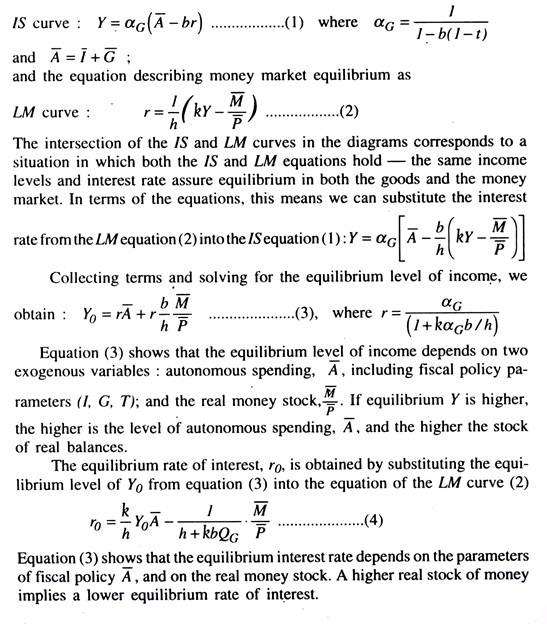
The intersection of the IS and LM curves determines equilibrium income and interest rate. We derive expressions for these values by using the equations of IS and LM curves.