Elasticity of Demand (With Example and Diagram)

In this article we will discuss about Elasticity of Demand:- 1. Concept of Elasticity of Demand 2. Types of Elasticity of Demand.

Concept of Elasticity of Demand:

In reality we often come across one or two sur­prising facts. For example, we observe that an in­crease in supply of an agricultural commodity, be­cause of a bumper crop or import of cheap corn from abroad, is likely to reduce its price. This fall in price is unlikely to raise demand because consump­tion of stable agricultural crops remain more or less unchanged in all situations.

So large output of any agricultural crop tends to be associated with low revenue (= P x Q) of the farmers. To understand this peculiar phenomenon we must learn an important economic concept, viz., ‘elasticity of demand’. Busi­ness firms, desirous of reducing prices in order to sell more of goods and services, and making more profit by doing so, must also be interested in the concept of elasticity.

And when a government department al­lows a public utility concern like the Calcutta Cor­poration to raise its price of water, or the Calcutta Electric Supply Corporation to raise the electricity tariff in order to wipe out its losses, the elasticity concept is very much involved.

The de­mand for a commodity depends on a number of vari­ables like the price of the commodity, the income of the buyers, prices of related goods and son on.

Consumers do respond to a change in one of the vari­ables affecting demand, other variables remaining unchanged. The elasticity of demand measures the responsiveness of the market demand for a commod­ity to a change in one of the variables affecting de­mand.

The concept of elasticity is extremely useful in any business situation. It is often made use of by marketing managers to set prices of various prod­ucts and services.

It is also used by a discriminating monopolist like the Calcutta Electric Supply Cor­poration to set different prices for the same com­modity in two different markets. The Finance Min­ister also makes use of the concept to explore the possibility of raising revenue by imposing sales tax or excise duty on a wide variety of goods.

There are two other concepts of elasticity, viz., market share elasticity and promotional elasticity (or advertisement elasticity of sales). The former measures the responsiveness of the percentage share one firm has of the market, to changes in the ratio of its prices to industry prices. The latter measures the responsiveness of sales to change in advertising or any other sales promotion outlay.

In other words, it is a measure of market sen­sitivity of demand. And there are three types of demand elasticity’s, viz., price elasticity, income elasticity and cross elasticity.

Types of Elasticity of Demand:

I. Price Elasticity of Demand:

Price elasticity is “a concept for measuring how much the quantity demanded responds to changing price”. In other words, “it is a relative measure of the responsiveness of changes in quantity demand­ed, the dependent variable, to changes in price, the independent variable”. In fact, various commodi­ties differ in the degree to which the quantity de­manded will respond to changes in their respective prices.

If the price of salt falls by 1% the quantity of salt demanded may go up by less than 1%. But the sales of colour TV sets may rise more than 1% for every 1% price cut. We can also think of an in­termediate situation where 1% cut in price may lead to exactly 1% increase in sales when per­centage change in price balances percentage chang­es in quantity.

The first case is one of weak percentage response of Q to changes in P and if this is the case demand is said to be inelastic. The second case is of strong percentage response of Q to changes in P and falls in the category of elastic demand. The intermediate (borderline) case is one of ‘unitary elasticity of de­mand.

The Total Revenue Test:

The conventional way of measuring elasticity is to look at the effect of price changes on the total revenue of business firm (or total expenditure of consumers). Total revenue is P x Q. If consumers buy 10 litre of petrol at Rs. 8 per litre, the total revenue is Rs. 80.

It is possible to see whether demand is elastic, unitary elastic or inelastic by examining the effect on total revenue of a price cut along the same de­mand curve:

Price elasticity is a measure of the degree of re­sponsiveness of quantity demanded of a commodity to changes in its market price. We can think of the following three alternative categories of price elasticity.

1. When percentage cut in P results in such a large change in Q that TR = (P x Q) rises, de­mand is said to be elastic (i.e., P₁Q₁ > P₀Q₀.)

2. When a percentage cut in P results in exactly the same percentage increase in Q so that TR remains unchanged (i.e., P₁Q₁ = P₀Q₀), demand is said to be unitary elastic.

3. When a percentage cut in P results in such a small percentage increase in Q that TR falls (i.e., P₁Q₁ < F₀Q₀) demand is said to be inelas­tic. The three figures below illustrate the three situations.

See also the following table which is self- explanatory.

The concept of elasticity has practical rele­vance. By using the concept in the business world, or in the labour market or in the Ministry of Finance (Government of India) it is possible to determine the sensitivity of changes in quantity demanded to changes in price. However, application of the con­cept is possible only after calculation of an elastici­ty coefficient.

Calculation of Price Elasticity:

Elasticity can be calculated in two ways. Firstly it as an average value over some range of the de­mand function, in which case it is called arc elas­ticity.

The arc price elasticity can be calculated us­ing the following mid-point formula:

Arc price elasticity of demand

The formula for calculating arc elasticity may be expressed as:

in which E_p is arc elasticity of quantity demanded with respect to price,

P₁ and Q₁ are the original price and quantity,

P₂ and Q₂ are the final price and quantity,

∆P is the absolute change in price and

∆Q is the absolute change in quantity.

Note that E_p is always a pure number like 1, 1/2, 1/ 4 etc.. because it is the ratio of two percentage changes.

Since the demand curve is downward sloping, either ∆P or ∆Q will be negative. Therefore, the calculated value for elasticity has negative sign.

On the basis of mid-point formula we may com­pute arc price elasticity. If E_p > 1 demand is said to be elastic; if E_p = 1 demand is unitary elastic and it E_p < 1 demand is inelastic. Consider the following example.

Example 1:

Suppose income is constant at Rs. 3,000 per year, present price of a good is Rs. 10 and present quantity demanded is 125 units per month. Now the price falls to Rs. 9 and a large quantity of 150 units per month is likely to be demanded. What is the arc price elasticity over this range of the demand curve?

Solution:

Substituting values into the arc elasticity for­mula, we get:

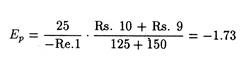
What is the significance of the calculated elastici­ty coefficient? It simply indicates that quantity ex­pands by 1.73% for each 1% fall in price over the relevant range of the demand curve. The negative value of the coefficient of demand elasticity sim­ply implies that quantity Q goes up when P falls and vice-versa.

The virtue of this method of calcu­lation is that it is a more accurate measure than if we had used the initial or final P and Q bases. This is because, when we deal with a range over which the price varies, it is always better to obtain a measure that reflects the average degree of consu­mer responsiveness.

For discrete (big) or once-for-all P change, we make use of the above formula. However, as a spe­cial case of arc elasticity we may use the concept of point elasticity. For small (or continuous) P and Q changes, E_p can be calculated for a point on the de­mand function, so as to be called point price elastic­ity.

Point Price Elasticity:

The responsiveness of quantity demand to price can alternatively be determined for a point on the demand function provided its slope is known to us. If we make P and Q changes smaller and smaller, at the limit, ∆Q/∆P becomes δQ/δP, the partial de­rivative of the demand equation with respect to price (holding other variables constant).

The formula used for calculating point elastici­ty (i.e., elasticity at a particular point of the de­mand curve) is expressed as follows:

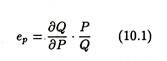
in which e_p is the point price elasticity of quantity demanded with respect to price, P and Q are any price and quantity chosen arbitrarily.

Example 2

The demand curves of commodities x and y are given by P_x = 6- 0,8q_x and P_y = 6 – 0.4q_y respectively. Show that at any given price, the two curves have the same elasticity of demand.

Solution:

We know elasticity of demand

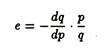
Now, the demand function of commodity x is p_x = 6 – 0.8 q_x

Example 3:

You have the sole authority to sell sandwiches in Eden Gardens during a test Match. Each costs 50 p. (including all relevant costs such as that of your labour).

From previous experience your best esti­mate of the demand is the following:

Calculate the elasticity of demand on this de­mand schedule around the price of Re. 1. Explain precisely the concept of elasticity you use.

Solution:

Elasticity of demand around a price of Re. 1:

Elasticity of demand =

Proportionate change in quantity demanded/Proportionate change in price

When price increases from Re. 1 to Rs. 1.05, propor­tionate increase is 5%. At Rs. 1.05 proportionate decrease in quantity demanded, i.e., from 2000 to 1800 is of 10%.

Elasticity of demand:

Conversely if price decreased from Re. 1 to 95 p., there is a decrease of 5%. At 95 p. quantity de­manded increases from 2000 to 2200, an increase of 10%.

.^.. Elasticity of demand = 10%/5% = 2

Since we get the same result for price increase and price fall, we need not use the mid-point formula.

Example 4

Consider the following equation relating the number of passengers (road users) per year on a rap­id transit system to the fare charges:

Q = 2207 – 52.4P (10.2)

in which Q = number of passenger per year

P = fare in paise

The partial derivative of the function with respect to price is:

Suppose a subsidized price of 10 paise per trip is of­fered to children below 2 years of age and the quan­tity at the subsidized price is : 1683 (millions).

Substituting the values into equation (10.2) we get

The coefficient of price elasticity – 0.31 simply im­plies that passenger traffic would fall by 0.31% for each 1% rise in fares.

II. Income Elasticity of Demand:

So long we have examined the responsiveness of changes in quantity demand to changes in price. But in reality the quantity demanded of a commodity also depends on the income of the buyer, which may refer to personal income or disposable income or national income, or per capita income.

The de­mand for meat, for example, depends on disposable personal income (i.e., personal income after paying all taxes). This variable is of greatest significance in determining the responsiveness of changes in quantity demanded of almost all consumer durable goods like cars, bicycles, T.V. sets, refrigerators, etc.

Income elasticity may be defined as the respon­siveness of changes in Q to a change in the income of the buyer(s). The coefficient of arc elasticity may be expressed as

It may be noted that the demand for a particu­lar commodity may be price elastic but income ine­lastic. For example, the demand for V.C.R. or T.V. sets or cars may be price inelastic but income elas­tic. If this is true, a marginal drop in the price of these items is unlikely cause a fall in the quantity demanded of those items, whereas an increase in income would lead to an increase in the number of V.C.R. T.V., or cars demanded.

In general price elasticity of demand for cars in developing coun­tries like India is found to be very high, whereas the income elasticity of demand is unitary. The im­plication is that a fall in the price of cars will lead to a sharp rise in the number of cars demanded. This will occur whether the economy is in the ex­pansionary or contractionary phase of the business cycle.

The numerical value of the co-efficient of in­come elasticity may be zero, positive, or negative. There may be a particular commodity like salt the quantity demanded of which may not respond to a small change in the income of the buyers. It is posi­tive in case of normal goods and negative in case of inferior goods.

If the quantity demanded of a commodity rises (falls) with an increase in income, the commodity is called a normal (inferior) good. Even in case of the same commodity – the coefficient of income elasticity may vary at different levels of income. See Figure 10.12.

Here Y_d is the income de­mand curve showing the relationship between Y_d (disposable income) and Q. At low levels of income (for income range OY₀) demand is elastic. Subse­quently it becomes completely inelastic (for income range Y₀ – Y₁). Finally, at higher levels of income Y₁ and above) demand is inelastic again.

Practical Relevance:

The concept of income elasticity has practical relevance. In fact, in order to determine the effect of changes in business activity, the business econo­mist must have a knowledge of income elasticities. On the basis of forecast of national or disposable personal income it is possible to apply income elas­ticities in estimating the changes in the purchases of consumer goods (especially durables).

However, such forecasts have limited value for two reasons:

(1) Sales are influenced by various other factors not included in the elasticity measure and

(2) The past pattern of purchase of a commodity is not an accu­rate indicator of the future.

III. Cross-Elasticity of Demand:

Cross elasticity of demand measures the inter­relationship of demand. In reality, the quantity demanded of a commodity, say motor cars, depends not only on its own price but also on the prices of fuel, tyres, mopeds, scooters, etc. Cross-elasticity measures the responsiveness of the quantity de­manded of a commodity to a change in the market price of another commodity.

The following formula is used to find out the numerical value of the elas­ticity coefficient:

in which P₁ and P₂ represent the new and old prices of the other commodity.

Likewise point cross-elasticity is measured by the formula:

The coefficient of cross elasticity can be zero, posi­tive or negative. It is zero in case of unrelated goods like tractors and motor cars. It is positive if the two commodities are substitutes.

For instance, an in­crease in the price of a substitute (say coffee) in­creases the quantity of the original commodity (say tea) demanded. Finally, it is negative if the two goods are complimentary. An increase in the price of petrol, for example, reduces the number of cars demanded.