Equilibrium of the Consumer (With Equations)

In this article we will discuss about:- 1. The Assumptions Equilibrium of the Consumer 2. Determination of the Equilibrium Purchase Plan 3. First-Order or Necessary Condition for Consumer Equilibrium  4. Economic Interpretation of the First-Order Conditions for Consumer Equilibrium 5. The Second-Order or Sufficient Condition for Consumer Equilibrium 6. Consumer Equilibrium – the Stability Considerations.

The Assumptions Equilibrium of the Consumer:

In analysing the equilibrium of the consumer, shall assume:

(i) Indifference curves.

(ii) The budget line of the consumer.

(iii) The consumer is a rational human being.

He tries to maximise the level of utility by spending all his money income on the two goods, X and Y. He would be in equilibrium only when he has been able to maximise utility subject to his budget constraint.

Determination of the Equilibrium Purchase Plan:

Let’s see how the consumer finds his equilibrium purchase plan with the help of Fig. 6.8. In this figure, his budget line LM upon his indifference map is superimposed. The consumer is able to purchase with his money income any combination of goods that lie on his budget line.

Remember here that at all the points on the budget line, the consumer’s expenditure is the same being equal to his money income. But at all these points his level of utility is not the same. For example, at both the points H and G on the budget line, the consumer spends all his money income, but he derives a higher level of utility from G because G is on a higher IC.

The consumer wants to find the point on LM which takes him to the highest possible IC. He may start from the point M and move northwestward along his budget line. In the process he moves on to higher and higher ICs at the points H, G, F, etc. and ultimately on to the highest possible IC₁ viz., IC₄, at the point E.

For if the consumer moves beyond the point E, he would be on the lower and lower ICs at the points T, S, R, etc. Instead of moving northwestward along his budget line, the consumer may very well start from the point L and move southeastward along his budget line. Here also he would be on the highest possible IC at the point E on IC₄.

It is evident in Fig. 6.8 that the consumer cannot reach a higher IC than IC₄ while moving along his budget line, because the line does not touch or cut any of these ICs. Therefore, the point E is the equilibrium point of the consumer where he would be able to maximise the level of utility subject to his budget constraint.

First-Order or Necessary Condition for Consumer Equilibrium:

Since the equilibrium point E is the point of tangency between the budget line and one of the ICs of the consumer, deduce the condition for consumer equilibrium in the following way. At the point E, the numerical slope of the IC = the numerical slope of the budget line

 

 

 

 

 

 

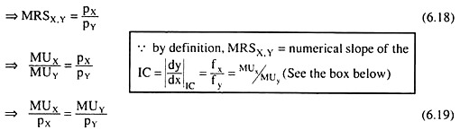
Equation (6.18) and (6.19) give two different forms of the first-order or necessary condition for consumer equilibrium.

Economic Interpretation of the First-Order Conditions for Consumer Equilibrium:

First analyse the economic significance of condition (6.18) which is

MRS_X,Y = p_X/p_Y

The economic significance of (6.18) would be obtained if it is remembered what the terms on the two sides of the equation stand for. By definition, MRS_X,_Y is the quantity of good Y that the consumer would be willing to forego for having an additional unit of X, provided his level of utility remains the same.

In other words, it is the significance to the consumer of the marginal unit or an additional unit of X in terms of Y. p_x/p_y on the other hand, is the price of a unit of X in terms of Y in the market.

Therefore, (6.18) states that, at the point of utility maximisation, significance of the marginal unit of X in terms of Y to the consumer should be equal to the price of the marginal unit of X in terms of Y in the market.

To illustrate the point, suppose, the price of X is Rs 10 and the price of Y is also Rs 10. Therefore, the price of an additional unit of X is 1 unit of Y—if the consumer wants to buy an additional unit of X in the market he would have to forego the purchase of 1 unit of Y.

Also suppose that the significance to him of One additional unit of X in terms of Y is more than 1 (unit of Y), it is equal to 5, say. In this case, good X would seem to be quite cheap to the consumer, because he is willing to forego 5 units of Y for having one more unit of X while the market price of X is 1 unit of Y.

A situation of this type would be obtained at a point, say, F, on the budget line in Fig. 6.9 which lies northwestward of the point of tangency E. At the point F, the numerical slope (steepness) of the IC, viz., IC₂, is larger (say 5) than that of the budget line (which is 1 = constant).

Since X would seem to be quite cheap at the point F, and Y quite costly (marginal significance of Y = 1/5 being less than market price of Y), the consumer in order to maximise his level of utility, would not settle at the point F.

He would rather want to buy more of X and less of Y, i.e., he would move downward towards right along his budget line till he reaches the point of tangency E where the marginal significance of good X to him would become equal to the market price of X, both being equal to 1 in terms of good Y.

On the other hand, at any point like G on the budget line downward towards right of E, which lies also on IC₁ the numerical slope of the IC (i.e., IC₁) is smaller than that of the budget line. Therefore, at G, market price of good X in terms of Y would be larger than the marginal significance of good X to the consumer in terms of good Y.

Now quite the opposite of what happened at point F, would be obtained. Now the consumer would find good X rather costly and good Y rather cheaper.

He would therefore be moving northwestward along his budget line leaving the point G, thereby decreasing his purchase of X and increasing his purchase of Y, till he reaches the point E where marginal significance of X (or Y) in terms of Y (or X) would become equal to the market price of X (or Y) in terms of Y (or X).

From the analysis, it is now clear that, in Fig. 6.9, the consumer would not purchase at any point on his budget line other than the point E. If he is not at point E, he would appropriately adjust and ultimately he would be in equilibrium at point E.

At the point E, which is the point of tangency, marginal significance of each good would become equal to its market price. That is why once he reaches E, he would show no tendency to move away from it.

Now look into the economic significance of condition (6.19) for consumer equilibrium. This condition is MU_X/p_X = MU_Y/p_Y.

These conditions are obtained as equation in the analysis of consumer equilibrium in the Marshallian utility theory. There it is seen that MU_X/P_X and MU_Y/P_Y are MU of money spent on goods X and Y, respectively.
It is also seen why the equality between MU of money spent on each good is required for utility-maximisation by the consumer.

It is not necessary to repeat those arguments. However, remember a major difference between the Marshallian analysis and the present analysis. In the former case, MU is measured cardinally in terms of money whereas in the latter case, MU is measured in terms of ordinal utility numbers.

The Second-Order or Sufficient Condition for Consumer Equilibrium:

The first-order condition (FOC) for consumer equilibrium is also called the necessary condi­tion. For example, it is necessarily required for the consumer to be in equilibrium that the MU of money spent on each good should be the same or the marginal significance of each good to the consumer should be equal to its market price.

If these requirements are not fulfilled, the consumer would have a tendency to move to other positions.

However, although necessary, the FOC is not a sufficient condition, even if the requirements of FOC are satisfied, the consumer may not be in utility-maximising equilibrium. For example, if the ICs are concave to the origin, the point of tangency between the consumer’s budget line and one of his ICs is the point where the FOC is satisfied, but at this point the consumer does not maximise his level of utility.

In fact, at this point, his level of utility is the minimum subject to his budget. This is evident in Fig. 6.10 where the ICs are concave to the origin and the budget line LM takes the consumer to the lowest possible IC at the point of tangency H.

As the consumer moves from H towards either direction along his budget line he reaches successively higher ICs. Therefore, although the FOC for consumer equilibrium has been satisfied at point H, this is not sufficient for the consumer to be in utility-maximising equilibrium.

If the ICs are convex to the origin, the budget line takes the con­sumer on to the highest possible IC at the point of tangency. It may be concluded, therefore, that for the utility maximising equilibrium of the consumer, ‘point of tangency’ is the first-order or necessary condition and the convexity (to the origin) is the second-order condition, or, sufficient condition.

Consumer Equilibrium – the Stability Considerations:

The two important forms of the first-order condition (FOC) for consumer

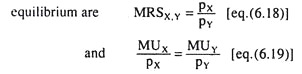
Also, the second-order condition (SOC) requires that the ICs should be convex to the origin. Now it is seen without much difficulty that the equilibrium of the consumer as guaranteed by the FOC and the SOC, is a stable equilibrium. For here if, for some reasons, the con­sumer is at an out-of-equilibrium point, then he would be driven by some forces or considera­tions to the equilibrium point.

Let’s consider again Fig. 6.9. In this figure, the consumer would be in equilibrium at the ‘point of tangency’ E. But if the consumer is at a disequilibrium point like F which lies northwestwards of point E on his budget line LM, then the numerical slope of the IC (viz., IC₂) at point F > the numerical slope of the budget line

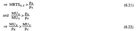
(6.21) gives, at point F, marginal significance of good X in terms of good Y is greater than market price of X in terms of Y, and (6.22) gives the MU of money spent on X is more than MU of money spent on Y. Therefore, the consumer would want to buy more of X and less of Y and he would be moving downwards towards right along his budget line till he reaches the equilibrium point E.

Similarly, if the consumer is at a disequilibrium point like G on his budget line, then the numerical slope of his IC (viz., IC₁) < the numerical slope of the budget line. Therefore, now, the opposite of what had happened earlier would be obtained, and the con­sumer would be moving upward towards left along his budget line till he reaches the equilib­rium point E.

If the consumer is not in equilibrium for some reasons, then forces would be there that would drive him to the equilibrium point. That is why it can be said that consumer equilibrium as ensured by the FOC and the SOC is a stable equilibrium.