The below mentioned article provides quick notes on the Fiscal Policy for Stability.
Two important tools of fiscal policy are G and T.
These two instruments can be varied to offset the effects of undesirable changes in private investment spending, which is the most volatile component of aggregate demand (desired expenditure).
The government can make appropriate use of G and T to stabilise total autonomous expenditure (C + I + G) and, therefore, equilibrium income even if I shows sudden and unexpected fluctuations.
ADVERTISEMENTS:
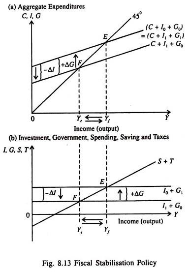
Fig. 8.13 shows the effect of fiscal policy. The economy is assumed I, G, S, T to be in equilibrium at a potential level Y̅f with aggregate demand equal to (C + I0 + G0). Now let us suppose autonomous investment schedule suddenly falls from I0 to I1, due to the fact that the marginal efficiency of capital receives a severe jolt. As a result, aggregate demand falls to (C + I1, + G0). The new equilibrium level of income (Y̅e) is now below its potential level.
Now the government can increase its own expenditure by an amount just sufficient to restore equilibrium at Y̅f. In Fig. 8.13, a rise in government expenditure by ΔG, i.e., to G0, shifts the aggregate demand curve back to its original position, so that the level of aggregate demand is now C + I1, + G1.
Thus, by increasing G, the economy is enabled to reachieve its potential level of output. The fall in I is completely offset by an increase in G, so as to keep C + I + G constant.
ADVERTISEMENTS:
Alternatively, the same effect may be achieved by cutting taxes. Since the tax multiplier is less than the government expenditure multiplier, the appropriate tax cut would be larger than the required increase in government expenditure. Part (b) of Fig. 8.13 shows that the fall in I + G by ΔI is offset by a rise in I + G by ΔG so that equilibrium income, after falling from Y̅f to Y̅e comes from Y̅e to Y̅f.
In short, a compensatory increase in G shifts the I + G schedule upward to its original position I1 + G1, and enables the economy to attain point E from which it moved to F due to fall in I.
This is an example of discretionary fiscal policy, because the government deliberately increases G or reduces T so as to enable the economy to move back from point F to E, at which the original equilibrium level of income Y̅f is restored.
