Single Decision of the Firm (With Diagram)

Single Decision of the Firms: Choice of Optimal Combination of Factor of Production!

In this section we shall show the use of the production function in the choice of the optimal combination of factors by the firm.

In Part A we will examine two cases in which the firm is faced with a single decision, namely maximizing output for a given cost, and minimizing cost subject to a given output.

Both these decisions comprise cases of constrained profit maximization in a single period. In Part B we will consider the case of unconstrained profit maximization, by the expansion of output over time.

In all the above cases it is assumed that the firm can choose the optimal combination of factors, that it can employ any amount of any factor in order to maximize its profits. This assumption is valid if the firm is new, or if the firm is in the long-run. However, an existing firm may be coerced, due to pressure of demand, to expand its output in the short-run, when at least one factor, usually capital, is constant. We will examine this case separately.

In all cases we make the following assumptions:

1. The goal of the firm is profit maximization – that is, the maximization of the dif­ference Π = R — C where

Π = profits

R = revenue

C – cost

2. The price of output is given, P_x.

3. The prices of factors are given

w is the given wage rate

r is the given price of capital services (rental price of machinery).

A. Single Decision of the Firm:

The problem facing the firm is that of a constrained profit maximization, which may take one of the following forms:

(a) Maximize profit Π, subject to a cost constraint. In this case total cost and prices are given (C, w, r, P_x), and the problem may be stated as follows

max Π = R — C

Π = P_xX – C

Clearly maximization of Π is achieved in this case if X is maximized, since C and P_x are given constants by assumption.

(b) Maximize profit Π, for a given level of output. For example, a contractor wants to build a bridge (X is given) with the maximum profit. In this case we have

max Π = R — C

Π = P_xX – C

Clearly maximization of Π is achieved in this case if cost C is minimized, given that X and P_x are given constants by assumption.

The analysis will be carried out first by using diagrams and subsequently by applying calculus.

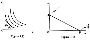
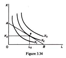
For a graphical presentation of the equilibrium of the firm (its profit-maximizing posi­tion) we will use the isoquant map (figure 3.32) and the iso-cost-line(s) (figure 3.33).

The slope of an isoquant is

where w = wage rate, and r = price of capital services.

The isocost line is the locus of all combinations of factors the firm can purchase with a given monetary cost outlay.

The slope of the isocost line is equal to the ratio of the prices of the factors of production

slope of isocost line = w/r

Assume that the total cost outlay the firm undertakes is C. If the entrepreneur spends all the amount C on capital equipment, the maximum amount he can buy from this factor is

0A = C / r

If all cost outlay is spent on labour the maximum amount of this factor that the firm can pur­chase is

0B = C/w

The slope of the isocost line is

0A/0B = C/r / C/ w = w/r

It can be shown that any point on the line AB satisfies the cost equation (C = r. K + w. L), so that, for given prices of the factors and for given expenditure on them, the isocost line shows the alternative combinations of K and L that can be purchased by the firm. The equation of the isocost line is found by solving the cost equation for K

K = C/r – w/ r L

By assigning various values to L we can find all the points of the isocost line.

Case 1: maximisation of output subject to a cost constraint (financial constraint):

We assume: (a) A given production function

X = ƒ(L, K, v, y)

and (b) given factor prices, w, r, for labour and capital respectively.

The firm is in equilibrium when it maximizes its output given its total cost outlay and the prices of the factors, w and r.

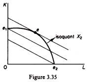
In figure 3.34 we see that the maximum level of output the firm can produce, given the cost constraint, is X₂ defined by the tangency of the isocost line, and the highest iso- quant. The optimal combination of factors of production is K₂ and L₂, for prices w and r. Higher levels of output (to the right of e) are desirable but not attainable due to the cost constraint. Other points on AB or below it lie on a lower isoquant than X₂.

Hence X₂ is the maximum output possible under the above assumptions (of given cost outlay, given production function, and given factor prices). At the point of tangency (e) the slope of the isocost line (w/r) is equal to the slope of the isoquant (MPJMP_K). This constitutes the first condition for equilibrium. The second condition is that the isoquants be convex to the origin.

In summary the conditions for equilibrium of the firm are:

(a) Slope of isoquant = Slope of isocost

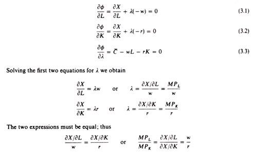
(b) The isoquants must be convex to the origin. If the isoquant is concave the point of tangency of the isocost and the isoquant curves does not define an equilibrium position (figure 3.35).

Output X₂ (depicted by the concave isoquant) can be produced with lower cost at e- which lies on a lower isocost curve than e. (With a concave isoquant we have a ‘corne solution.)

Formal derivation of the equilibrium conditions:

The equilibrium conditions may be obtained by applying calculus and solving a ‘constrain maximum’ problem which may be stated as follows. The rational entrepreneur seeks the ma misation of his output, given his total-cost outlay and the prices of factors.

Formally:

Maximise X =ƒ (L, K)

subject to C = wL + rK (cost constraint)

This is a problem of constrained maximum and the above conditions for the equilibrium of firm may be obtained from its solution.

We can solve this problem by using Lagrangian multipliers.

The solution involves the follow steps:

Rewrite the constraint in the form

C – wL – rK = 0

Multiply the constraint by a constant λ which is the Lagrangian multiplier

λ(C – wL – rK) = 0

The Lagrangian multipliers are undefined constants which are used for solving constrain maxima or minima. Their value is determined simultaneously with the values of the o^th unknowns (L and K in our example). There will be as many Lagrangian multipliers as there are constraints in the problem. Form the ‘composite’ function

ɸ = X + λ(C- wL – rK)

It can be shown that maximization of the ɸ function implies maximization of the output.

The first condition for the maximization of a function is that its partial derivatives be equal to zero.

The partial derivatives of the above function with respect to L, K and λ are:

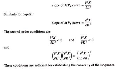
This firm is in equilibrium when it equates the ratio of the marginal productivities of factors to the ratio of their prices. It can be shown that the second-order conditions for equilibrium of the firm require that the marginal product curves of the two factors have a negative slope.

The slope of the marginal product curve of labour is the second derivative of the production function:

Case 2: Minimisation of cost for a given level of output:

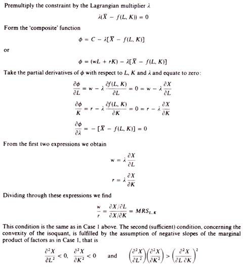
The conditions for equilibrium of the firm are formally the same as in Case 1. That is, there must be tangency of the (given) isoquant and the lowest possible isocost curve, and the isoquant must be convex. However, the problem is conceptually different in the case of cost minimization. The entrepreneur wants to produce a given output (for example, a bridge, a building, or X tons of a commodity) with the minimum cost outlay.

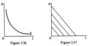
In this case we have a single isoquant (figure 3.36) which denotes the desired level of output, but we have a set of isocost curves (figure 3.37). Curves closer to the origin show a lower total-cost outlay. The isocost lines are parallel because they are drawn on the assumption of constant prices of factors: since w and r do not change, all the isocost curves have the same slope w/r.

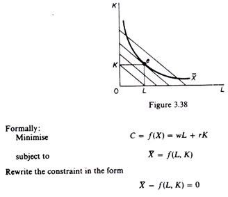
The firm minimizes its, costs by employing the combination of K and L determined by the point of tangency of the X isoquant with the lowest isocost line (figure 3.38). Points below e are desirable because they show lower cost but are not attainable for output X. Points above e show higher costs. Hence point e is the least-cost point, the point denoting the least-cost combination of the factors K and L for producing X.

Clearly the conditions for equilibrium (least cost) are the same as in Case 1, that is, equality of the slopes of the isoquant and the isocost curves, and convexity of the isoquant.

B. Choice of Optimal Expansion Path:

We distinguish two cases: expansion of output with all factors variable (the long run), and expansion of output with some factor(s) constant (the short run).

Optimal expansion path in the long run:

In the long run all factors of production are variable. There is no limitation (technical or financial) to the expansion of output. The firm’s objective is the choice of the optimal way of expanding its output, so as to maximize its profits. With given factor prices (w, r) and given production function, the optimal expansion path is determined by the points of tangency of successive isocost lines and successive isoquants.

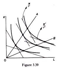
If the production function is homogeneous the expansion path will be a straight line through the origin, whose slope (which determines the optimal K/L ratio) depends on the ratio of the factor prices. In figure 3.39 the optimal expansion path will be 0A, defined by the locus of points of tangency of the isoquants with successive parallel isocost lines with a slope of w/r.

If the ratio of the prices increases the isocost lines become flatter (for example, with a slope of w’/r’), and the optimal expansion path will be the straight line 0B. Of course, if the ratio of prices of factors was initially w/r and subsequently changes to w’/r’, the expansion path changes initially the firm moves along 0A, but after the change in the factor prices it moves along 0B.

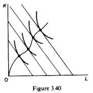
If the production function is non-homogeneous the optimal expansion path will not be a straight line, even if the ratio of prices of factors remains constant. This is shown in figure 3.40. It is due to the fact that in equilibrium we must equate the (constant) w/r ratio with the MRS_L,k, which is the same on a curved isocline.

Optimal expansion path in the short run:

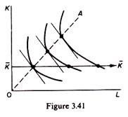
In the short run, capital is constant and the firm is coerced to expand along a straight line parallel to the axis on which we measure the variable factor L. With the prices of factors constant the firm does not maximize its profits in the short run, due to the constraint of the given capital. This situation is shown in figure 3.41. The optimal expansion path would be 0A were it possible to increase K. Given the capital equip­ment, the firm can expand only along KK in the short run.

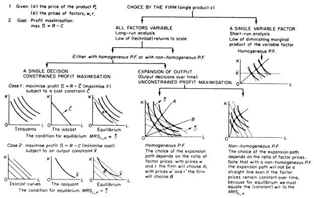
The above discussion of the choice of optimal combination of the factors of production is schematically summarised on p. 94.