Producer’s Equilibrium or Optimisation (With Diagram)

In this article we will discuss about Producer’s Equilibrium or Optimisation.

Producer’s equilibrium or optimisation occurs when he earns maximum profit with optimal combination of factors. A profit maximisation firm faces two choices of optimal combination of factors (inputs).

1. To minimise its cost for a given output; and

2. To maximise its output for a given cost.

Thus the least cost combination of factors refers to a firm producing the largest volume of output from a given cost and producing a given level of output with the minimum cost when the factors are combined in an optimum manner. We study these cases separately.

Cost-Minimisation for a Given Output:

In the theory of production, the profit maximisation firm is in equilibrium when, given the cost-price function, it maximises its profits on the basis of the least cost combination of factors. For this, it will choose that combination which minimizes its cost of production for a given output. This will be the optimal combination for it.

Assumptions:

This analysis is based on the following assumptions:

1. There are two factors, labour and capital.

2. All units of labour and capital are homogeneous.

3. The prices of units of labour (w) and that of capital (r) are given and constant.

4. The cost outlay is given.

5. The firm produces a single product.

6. The price of the product is given and constant.

7. The firm aims at profit maximisation.

8. There is perfect competition in the factor market.

Explanation:

Given these assumptions, the point of least-cost combination of factors for a given level of output is where the isoquant curve is tangent to an iso-cost line. In Figure 17, the iso-cost line GH is tangent to the isoquant 200 at point M.

The firm employs the combination of ОС of capital and OL of labour to produce 200 units of output at point M with the given cost-outlay GH. At this point, the firm is minimising its cost for producing 200 units.

Any other combination on the isoquant 200, such as R or T, is on the higher iso-cost line KP which shows higher cost of production. The iso-cost line EF shows lower cost but output 200 cannot be attained with it. Therefore, the firm will choose the minimum cost point M which is the least-cost factor combination for producing 200 units of output.

M is thus the optimal combination for the firm. The point of tangency between the iso-cost line and the isoquant is an important first order condition but not a necessary condition for the producer’s equilibrium.

There are two essential or second order conditions for the equilibrium of the firm:

1. The first condition is that the slope of the iso-cost line must equal the slope of the isoquant curve. The slope of the iso-cost line is equal to the ratio of the price of labour (w) to the price of capital (r) i.e… W/r. The slope of the isoquant curve is equal to the marginal rate of technical substitution of labour and capital (MRTS_LC) which is, in turn, equal to the ratio of the marginal product of labour to the marginal product of capital (MP_L/MP_C).

Thus the equilibrium condition for optimality can be written as:

W/r = MP_L/MP_C = MRTS_LC

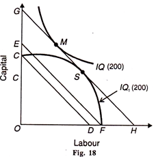
2. The second condition is that at the point of tangency, the isoquant curve must he convex to the origin. In other words, the marginal rate of technical substitution of labour for capital (MRTS_LC) must be diminishing at the point of tangency for equilibrium to be stable. In Figure 18, S cannot be the point of equilibrium, for the isoquant IQ₁ is concave where it is tangent to the iso-cost line GH.

At point S, the marginal rate of technical. substitution between the two factors increases if move to the right or left on the curve lQ₁ .Moreover, the same output level can be produced at a lower cost CD or EF and there will be a corner solution either at С or F. If it decides to produce at EF cost, it can produce the entire output with only OF labour. If, on the other hand, it decides to produce at a still lower cost CD, the entire output can be produced with only ОС capital.

Both the situations are impossibilities because nothing can be produced either with only labour or only capital. Therefore, the firm can produce the same level of output at point M where the isoquant curve IQ is convex to the origin and is tangent to the iso-cost line GH. The analysis assumes that both the isoquants represent equal level of output IQ = IQ₁ = 200.

Output-Maximisation for a given Cost:

The firm also maximises its profits by maximising its output, given its cost outlay and the prices of the two factors. This analysis is based on the same assumptions, as given above.

The conditions for the equilibrium of the firm are the same, as discussed above.

1. The firm is in equilibrium at point P where the isoquant curve 200 is tangent to the iso-cost line CL in Figure 19.

At this point, the firm is maximising its output level of 200 units by employing the optimal combination of OM of capital and ON of labour, given its cost outlay CL. But it cannot be at points E or F on the iso-cost line CL, since both points give a smaller quantity of output, being on the isoquant 100, than on the isoquant 200.

The firm can reach the optimal factor combination level of maximum output by moving along the iso-cost line CL from either point E or F to point P. This movement involves no extra cost because the firm remains on the same iso-cost line.

The firm cannot attain a higher level of output such as isoquant 300 because of the cost constraint. Thus the equilibrium point has to be P with optimal factor combination OM + ON. At point P, the slope of the isoquant curve 200 is equal to the slope of the iso-cost line CL. It implies that w/r = MP_L/MPC = MRTS_LC

2. The second condition is that the isoquant curve must be convex to the origin at the point of tangency with the iso-cost line, as explained above in terms of Figure 18.