
The balanced budget multiplier refers to the effects of an increase in government purchases accompanied by an increase in taxes such that in the new equilibrium, the budget surplus is exactly the same as in the original equilibrium.
The result is that the multiplier of such a policy change, the balanced budget multiplier, is equal to 1.
A multiplier of unity implies that output expands by precisely the same amount of the increased government purchases with no induced consumption spending. It should be clear that what must be at work is the effect of higher taxes that exactly offsets the effect of the income expansion, thereby maintaining disposable income, and hence consumption constant. With no induced consumption spending, output expands simply to match the increased government purchases.
That the value of balanced budget multiplier is equal to 1 can be shown formally by noting that the change in aggregate demand ∆AD is equal to the change in government purchases plus the change in consumption spending. The change in consumption spending is equal to the marginal propensity to consume out of disposable income, c, times the change in disposable income, ∆YD, that is, ∆YD = ∆Y0 – ∆TA, where ∆Y0 is the change in output and ∆TA is the change in taxes.
ADVERTISEMENTS:
Thus
![]()
We know that the change in aggregate demand has to equal the change in output as the economy moves from one equilibrium to another. So we have
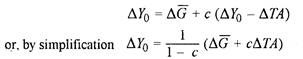
Next we must note that by assumption the change in government purchases between the new equilibrium and the old one is exactly matched by a change in tax collection under the balanced-budget policy. It follows that ∆G = ∆TA.
![]()
If we substitute this value of ∆TA in the relation (2), we have so that the balanced-budget multiplier is precisely unity. The change in income as a result of a given change in taxes in a balanced budget is equal to the change in taxes. But the analysis of balanced budget multiplier given above presumes that there are no money-market effects of the change in taxes (TA) and hence of ∆G. This is correct as long as we are in the domain of Keynes’s investment multiplier.
The value of balanced-budget multiplier becomes less than unity if we take the effect of ∆Y0 on the rate of interest. Hicks’s IS – LAI analysis is helpful in explaining the reduced value of the balanced-budget multiplier. It tells us that the change in taxes (TA) changes the disposable income in the hands of the public which in turn changes the demand for money for transactions purposes. Suppose that the ∆G is positive and therefore ∆Y0 is positive.
The demand for money accordingly goes up and pushes up the rate of interest in the money market which has a discouraging effect on private investment. Therein, the multiplier effect in play is truncated to the extent investment is restricted. This partially offsets the initial increase in income given as ∆Y0 that is less than the initial change in taxes (TA).
ADVERTISEMENTS:
We thus come to the conclusion that even a balanced-budget policy can have expansionary and contractionary effect on income. The traditional assumption of the neutrality of a balanced-budget policy in economic affairs stands questioned under the IS – LM analysis.
Dubious Assumptions:
The balance-budget multiplier theory is an integral part of fiscal policy. However, because of some questionable premises on which the theory is based, it has not gone without criticism.
In general, it can be said:
The balanced-budget multiplier theory rests on some dubious assumptions. Therefore, although it is logically correct within the Keynesian model, it may not always work as expected. For example, increased government spending and taxes may at times impede rather than stimulate the private sector’s growth. The effect of this will be to increase rather than to decrease unemployment and inflation. This helps to explain why it is not always possible to predict accurately what the consequences of fiscal policies would be.