Graphical Representation of Good Market through the IS-Curve

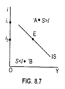
The IS curve shows the combination of interest rates and the income levels at which the goods market clears.

The product market is in equilibrium when:

Planned spending = Planned output

Or where Investment = Savings at different rates of interests.

Therefore, it is called ‘I equal S’ Or ‘I-S’ function.

Thus, IS curve is a graphic representation of the product market equilibrium condition.

The Investment Curve/Function:

Investment demand is an endogenous variable which depends on the rate of interest.

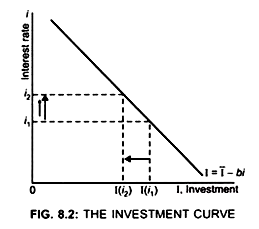
Equation (i) shows that the lower the interest rate, the higher is the planned investment, that is, there exists an inverse relationship between the interest rate and investment. This is because when the firms borrow to purchase investment goods, they have to pay an interest rate. When interest rate increases, the cost of borrowings increases.

This decreases the profitability of the firms and thus, the planned investment decreases. Due to this negative relationship between interest rate and the investment, the investment curve is negatively sloped. (Fig. 8.2) [I ↑, cost of borrowings ↑, I ↓]

Initially at interest rate i₁, Investment is I (i₁)

When interest rate increases from i₁ to i₂

Investment decreases from I (i₁) to I(i₂) (Fig. 8.2)

This shows that there exists inverse relationship between investment and interest rate.

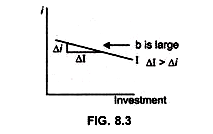
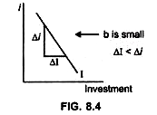
The slope of Investment curve (I = I – bi) depend on the value of b,

(i) If b is large then investment will be highly sensitive to interest rate

.^.. slope of I curve will be less, that is, Investment curve will be flatter. (Fig. 8.3)

(ii) If b is small, Investment curve will be steep

Derivation of IS Curve or Equilibrium in the Goods Market:

By selecting arbitrary rate of interest and then finding the income level which is consistent with each rate of interest we get the IS curve which has a negative slope because when interest rate falls, investment increases and thus income level increases. Thus IS curve is a locus of points showing equilibrium points of product market at various combinations of investment, saving, interest rate and income level.

(i) From the aggregate demand approach (C + I + G + NX) we have the following three equations to cover the goods market:

(ii) From the S, I approach we have the following three equations to cover the goods market:

Effect of interest rate on AD:

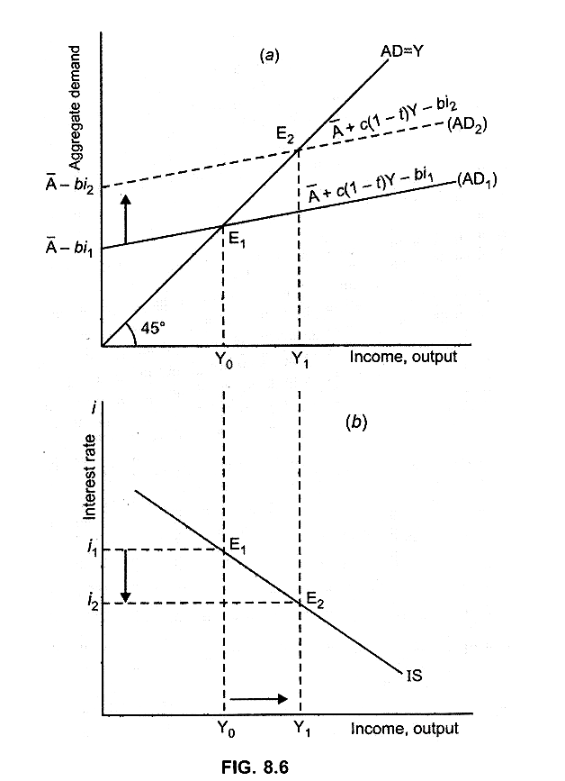
Change in interest rate leads to a change in the investment. Assume interest rate falls, this will lead to decease in cost of borrowings and therefore investment will increase. As investment is a component of AD, increase in investment will lead to a change, that is, increase in AD, which in turn leads to a change, that is, increase in income. Thus, a change in interest rate leads to a change in the equilibrium level of income.

Equilibrium condition: Y = AD

(i) Assume the interest rate is (i₁):

Product market is in equilibrium at point E₁ as here Y = AD₁, that is, AD₁ curve intersects the 45° line at point E₁ (Fig. 8.5a)

By plotting the combination (i₁, Y₀) in the lower panel we get point E₁.

This gives us one point on the IS curve, that is one combination of interest rate and income level where the goods market is in equilibrium.

(ii) Assume the interest rate falls to i₂:

Investment will increase because the cost of borrowing decreases.

As investment is a component of AD, an increase in investment will lead to an increase in AD. The intercept of AD will increase. The AD curve will shift parallel upward from AD₁ to AD₂ (Fig. 8.5a).

As a result income level will rise from Y₀ to Y₁.

Thus, decrease in interest rate to i₂ leads to an increase in income level to Y₁.

By plotting the pair (i₂, Y₁) we get point E₂, another combination of interest rate and income level where the goods market is in equilibrium.

(iii) Similarly, we can get a number of combinations of interest rates and income levels where the goods market is in equilibrium.

By joining points E₁ and E₂ we get the IS curve (Fig 8.5b).

Thus, the IS curve shows the combinations of interest rates and income levels such that the goods market is in equilibrium. The IS curve is negatively sloped because when the interest rate decreases, the planned investment increases, which in turn increases the AD and thus, the equilibrium income level increases.

(i) At any point to the right of IS curve e.g. point A →S > I (Fig 8.7).

Reason:

At point A: i₁ > i₀. Result: Investment will decrease. At the same time

Y at point A > Y at Point E.

As saving is positively related to Y.

.^.. S will increase. Thus, S > I.

(ii) At any point to the left of IS curve e.g. point B → S < I.

Therefore, product market equilibrium has to be only on the IS curve. At any point to the right or left of IS curve there will be disequilibrium.