Let us make an in-depth study of the Balanced Budget Multiplier. After reading this article you will learn about: 1. Determination of the Balanced Budget Multiplier in SKM 2. Derivation of the Balanced Budget Multiplier in SKM.
Determination of the Balanced Budget Multiplier in SKM:
According to Keynes, any increase in autonomous expenditure will have a multiplier effect.
So government expenditure, like autonomous investment also has a multiplier effect.
For instance, for a change in government expenditure (G), we have
![]()
Another policy-controlled element of autonomous expenditure is tax which is used to finance government expenditure. Although taxes depend on income or its change, since government expenditure is financed largely by taxes, the two variables — government expenditure and taxes (T) — are considered together while assessing the effect of G on Y.
For a change in taxes, we have
![]()
A one rupee increase in G has the same effect on equilibrium income as a one-rupee increase in I. Each implies a one-rupee increase in autonomous expenditure. So each has the same multiplier effect. In each case the initial increase in income generates induced increases in consumption, through the multiplier.
ADVERTISEMENTS:
The effect of an increase in G can be shown exactly in the same way as we have shown the effect of an increase in I. The C + I + G0 schedule will shift upward to C + I + G1, where G1 = G + ΔG. A diagram similar to Fig. 8.11 can be drawn to show this.
If ΔG = ΔI, ΔY will be the same because ΔY = 1/1-b(ΔG) = 1/1-b(ΔI), i.e., investment multiplier and government expenditure multiplier are equal. In this case the I + G schedule will shift upward from I0 + G0 to I0 + G1 where G1 – G0 = AG is the same as I1 – I0 = AI in Fig. 8.11 After all, both I and G are injections into the circular flow of income.

Since taxes, like savings, are a leakage from the circular flow of income, we see from equation (28) that the effect of an increase in taxes is in the opposite direction to those of increased G or I. An increase in taxes affects consumption spending by reducing disposable income (Y – T) at any level of national income.
ADVERTISEMENTS:
As a result the aggregate curve shifts downward at all levels of national income. In Fig. 8.12 we illustrate the effect of an increase in taxes on equilibrium income. If taxes rise by ΔT from T0 to T1, the aggregate curve shifts downward from (C + I + G)0 to (C + I + G)1 to equilibrium point F. This is due to downward shift of the consumption schedule caused by a rise in taxes. Equilibrium income falls from Y̅0 to Y̅1. The fall in income per rupee increase in taxes is equal to the tax multiplier -b/1 – b.
Thus if taxes rise by ΔT, equilibrium income falls by –(b 1-b)ΔT. In part (b) of Fig.8.12 we see that the saving plus taxes schedule shifts upward from S + T0 to S + T1. At the new equilibrium point F, national income Y1, is lower than it was at the original equilibrium point (i.e., Y0).
It may be noted that when the government imposes an additional tax of ΔT1, the aggregate demand schedule shifts down by (-ΔT), that is, by less ΔT since the MPC or (b) < 1. The reason is that, at a given level of income, a one-rupee increase in taxes reduces disposable income by one rupee but reduces consumption spending by less than one rupee since b < 1.
The rest of the fall in income by one rupee is absorbed by a fall in saving, by MPS (or S = 1 – b) times the fall in income. Since a one-rupee change in taxes shifts the aggregate curve by only a fraction (- b) of one rupee, the effect of a one-rupee increase in taxes on equilibrium income is -b times the autonomous expenditure multiplier, i.e., -b (1 1-b) = -b/1-b.
There is a relationship between the absolute values of tax and government expenditure multipliers, as the following examples show:
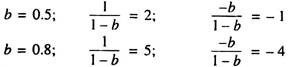
Thus we see that in each of the above two examples the tax multiplier is one less in absolute value than the government expenditure multiplier. This fact has an interesting implication for the effects of an equal increase in government spending and taxes, so that budgetary balance is maintained (ΔG = ΔT).
If we add the two multipliers in case of a balanced budget increase, i.e., an increase in G supported by an equal increase in T, we can find out the effects of such a combination of policy changes:
![]()
Thus we see that a one-rupee increase in G financed by a one-rupee increase in T increases equilibrium income by one rupee. This interesting result is known as the balanced budget multiplier, which brings into focus an interesting point: tax changes have a smaller per- rupee impact on equilibrium income than do changes in G or I.
ADVERTISEMENTS:
The value of the balanced budget multiplier, also called the unit budget multiplier, is 1 because the tax multiplier is always one less than the autonomous (government) expenditure multiplier.
This general result simply suggests that if both G and T increase by the same amount at the same time, so that the budgetary balance is maintained, equilibrium income increases exactly by the amount by which G and T increase in the first instance.
When the budget of the government is in balance, the government is said to be fiscally neutral. This means that fiscal policy has a neutral effect on the economy. But this is not true. Even in case of balanced budget increases, fiscal policy exerts considerable influence on the economy.
Derivation of the Balanced Budget Multiplier in SKM:
ADVERTISEMENTS:
The central government budget is in balance when current receipts are equal to current expenditure. Keynes, however, showed how the budgetary surpluses and deficits could be used to regulate the economy. However, a balanced budget does not necessarily have a neutral effect on the economy.
For instance, if the government raises taxes on the rich to give assistance to the poor, the budget would have a multiplier effect and generate additional incomes overall. This is because the propensity to save (consume) of the rich is higher (lower) than that of the poor.
Let investment change be some amount dl.
This change in investment will lead to some change in income dY by the formula:
ADVERTISEMENTS:
![]()
We know, that equation states that an increase in investment expenditure of Re. 1 will raise the level of income by Rs. 4, if the MPC (here b) is 0.75.
In the same way, we see that the change in income for equal changes in consumption, investment and government expenditures will be identical. Symbolically,
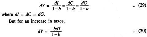
This means that taxes have a less strong effect on the level of income than do government expenditures. Taxes affect the level of income through their effect on consumption.
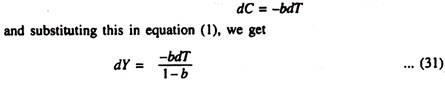
The change in income which results from a change in consumption is from equation (29):
ADVERTISEMENTS:
![]()
i.e., the change in consumption times the multiplier 1/(1 – b). The change in consumption resulting from a tax increase of dT is not equal to dT but is equal to the marginal propensity to consume, times dT. Thus, if the MPC is 0.75, a tax increase of Re. 1, by lowering disposable income by Re. 1, reduces consumption by 0.75 of Re. 1.
Therefore, we can write:
An increase in government expenditure of Rs. 20 crore raises aggregate demand by the same amount. But the level of income rises by
![]()
On the other hand, an increase in taxes of the same amount reduces consumption and aggregate demand by 0.75 x Rs. 20 crore = Rs. 15 crore and thus lowers the level of income by
![]()
The combined effect of the Rs. 20 crore increase in both taxes and government expenditure is therefore Rs. 80 crore – Rs. 60 crore = Rs. 20 crore, a value which is just equal to the change in G and T. This result is known as the “balanced budget” or “unit” multiplier theorem.
![]()
Cases where BBM ≠ 1:
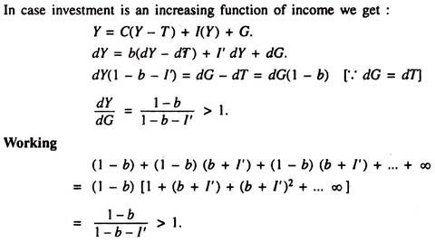
Output sensitivity of investment makes the multiplier effect stronger.
ADVERTISEMENTS:
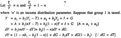
Now we consider two different income groups having different values of MPC:
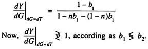
Suppose one group is taxed and the tax proceeds are used to finance government expenditure.
Total income is distributed between the two income groups: Y = Y1, + Y2.