Assumptions of the Law of Demand

Assumptions of Law of Demand as described by the Prof. Samuelson.

After reading this article you will learn about: 1. Assumptions of the Law of Demand 2. Fundamental Theorem or Demand Theorem.

Assumptions of the Law of Demand:

Samuelson’s law of demand is based on the following assumptions:

(1) The consumer’s tastes do not change.

(2) His choice for a combination reveals his preference for that.

(3) The consumer chooses only one combination at a given price-income line, i.e., any change in relative prices will always lead to some change in what he purchases.

(4) He prefers a combination of more goods to less in any situation.

(5) The consumer’s choice is based on strong ordering.

(6) It assumes consistency of consumer behaviour. If A is preferred to В in one situation, В cannot be preferred to A in the other situation.

This is the two-term consistency, according to Hicks which must satisfy two conditions on a straight line curve:

(a) If A is left to В, В must be right of A.

(b) If A is right of В В must be left of A.

(7) This theory is based on the assumption of transitivity. Transitivity, however, refers to three-term consistency. If A is preferred to B, and В to C, then the consumer must prefer A to C. This assumption is necessary for the revealed preference theory if the consumer is to make a consistent choice from given alternative situations.

(8) Income elasticity of demand is positive i.e., more commodity is demanded when income increases, and less when income falls.

Fundamental Theorem or Demand Theorem:

Given these assumptions, Samuelson states his “Fundamental Theorem of Consumption Theory,” also known as demand theorem, thus:

“Any good (simple or composite) that is known always to increase in demand when money income alone rises must definitely shrink in demand when its price alone rises.” It means that when income elasticity of demand is positive, price elasticity of demand is negative. This can be shown both in the case of a rise and a fall in the price of a good.

Rise in Price:

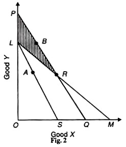
First, we take a rise in the price of, say, good X. To prove this Fundamental Theorem, let us divide it into two stages. Firstly, take a consumer who spends his entire income on two goods X and Y. LM is his original price-income line where the consumer is observed to have chosen the combination represented by R in Figure 2.

The triangle OLM is the consumer’s area of choice for the differ­ent combinations of X and Y available to him, as given by his price- income line LM.

By choosing only the combination R, the consumer is revealed to have preferred this combination to all others in or on the triangle OLM. Suppose the price of X raises the price of Y remaining constant so that the new price-income line is LS. Now he chooses a new combination, say, point A which shows that the consumer will buy less of X than before as the price of X has risen.

In order to compensate the consumer for the loss in his real income as a result of rise in the price of X, let us give him LP amount of money in terms of good К As a result, PQ becomes his new price-income line which is parallel to the LS line and passes through point R. Prof. Samuelson calls it Over Compensation Effect.

Now the triangle OPQ becomes his area of choice. Since R was revealed preferred to any other point on the original price-income line LM, all points lying below R on the RQ segment of PQ line will be inconsistent with consumer behav­iour.

This is because he cannot have more of X when its price has risen. The consumer will, therefore, reject all combinations below R and choose either combination R or any other combination, say, В in the shaded area LRP on the segment PR of the price-income line PQ. If he chooses the combination R, he will buy the same quantities of X and Y which he was buying before the rise in the price of X, On the other hand, if he chooses the combination B, he will buy less of X and more of Y than before.

In the second stage, if the packet of extra money LP given to the consumer is taken back, he will be to the left of R at point A on the price-income line LS where he will buy less of X, if the income elasticity of demand for X is positive. Since with the rise in the price of X, its demand has fallen (when the consumer is at point A), it is proved when income elasticity is positive, price elasticity is negative.

Fall in Price:

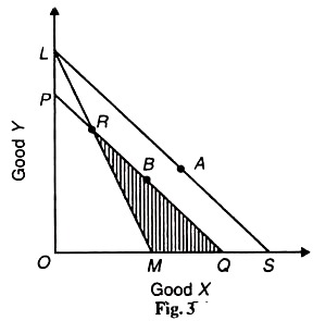
The demand theorem can also be proved when the price of good A^–falls. It can be defined thus: “Any good (simple or composite) that is known always to decrease demand when money income alone falls must definitely expand in demand when its price alone falls.” This is explained in Figure 3.

LM is the original price-income line on which the consumer reveals his preference at point R. With the fall in the price of X, the price of У remaining constant, his new price-income line is LS. The consumer reveals his preference on this line at, say, combination A which shows that he buys more of X than before.

The movement from point R to A is the price effect as a result of fall in the price of X which has led to increase in its demand.

Suppose the increase in the real income of the consumer as a result of fall in the price of X is taken away from him in the form of LP quantity of Y. Now PQ becomes his new price-income line which is parallel to LS and passes through R.

The new triangle OPQ becomes his area of choice. Since the consumer was revealing his preference at point R on the line LM, all points lying above R on the segment RP of line PQ will be inconsistent with his choice. This is because on the RP segment he will have less of good X when its price has fallen. But this is not possible.

The consumer will, therefore, reject all combinations above R. He will either choose combination R or any other combination, say, В on the segment RQ of the line PQ in the shaded area MRQ. If he chooses the combination R, he will buy the same quantities of X and Y which he was buying before the fall in the price of X.

And if he chooses the combination B, he will buy more of X and less of Y than before. The movement from R to В is the substitution effect of a fall in the price of X.

If the money taken from the consumer in the form of LP is returned to him, he will be at the old combination A on the price-income line LS where he will buy more of X with the fall in its price. The movement from В to A is the income effect. So the demand theorem is again proved that positive income elasticity means negative price elasticity of demand.

It is to be noted that Samuelson’s explanation of the substitution effect is different from that of the indifference curve analysis.

In the case of indifference curve analysis, the consumer moves from one combina­tion to another on the same indifference curve and his real income remains constant. But in the revealed preference theory, indifference curves are not assumed and the substitution effect is a movement along the price-income line arising from changing relative prices.