Inflation and Unemployment (With Diagram)

Let us make an in-depth study of the relationship of inflation with unemployment.

From AS to the Phillips Curve (PC):

A relationship between inflation and unemployment called the Phillips Curve which shows the short-run trade-off between inflation and unemployment implied by the short-run ASC. The PC is another way to express AS.

The short-run ASC shows a positive relationship between the price level and output. Since inflation is the rate of change in the price level and since unemployment fluctuates inversely with output, the ASC implies a negative relationship between inflation and unem­ployment. The PC expresses this negative relationship.

The PC points out that the inflation rate — the % change in the price level — depends on three forces:

(1) Expected inflation

(2) The deviation of unemployment from the natural rate, called cyclical unemployment.

(3) Supply shocks.

These forces can be expressed in the following equation

n = n_e — β (u — uⁿ) + ε

Inflation = Expected inflation-β(cyclical unemployment) + Supply Shock. Where β is a parameter greater than zero. Notice that, there is a minus sign before β which means high unemployment tends to reduce inflation.

From ASC to the Phillips Curve:

We can see that the ASC and Phillips curve express essentially the same relationship. The equation for the ASC is: P = P^e + (1/α) (Y – Y̅)………… (1) We can derive the Phillips curve from the equation of the ASC.

First, subtract last year’s price level P_-1 from both sides of the equation to obtain: (P – P_-1) = (P^e – P_-1) + (1/α) (Y – Y̅).

(P – P_-1) = Inflation π. (P^e – P_-1) = expected inflation, π^e. Thus, we can write equation as π = π^e + (1/α) (Y – Y̅).

Application of Okun’s law—which gives a relationship between output and unemployment—enables us to substitute – β (u – uⁿ) for (1/α)(Y- Y̅). Thus, the equation becomes: n – n^e – β (u – uⁿ). Here Okun’s law states that, the deviation of output from its natural rate is inversely related to the deviation of unemployment from its natural rate; that is, when output is higher than the natural rate of output, unemployment is lower than the natural rate of unemployment.

Finally, if a supply shock e is added to represent exogenous influence on prices, such as, a change in oil prices, a change in the minimum wage, etc., we get: n = n^e – β (u – uⁿ) + ε. Thus, we obtain the Phillip’s curve from the AS equation.

Now we can see that the PC retains the key feature of the short-run ASC, a link between real and normal variables that causes the classical dichotomy to fail. More precisely, the PC demonstrates the connection between real economic activity and unexpected changes in the price level. The PC is a convenient way to express and analyse AS.

Expectations and Inflation Inertia:

To make the PC useful, we need to say what determines expected inflation. A simple and often plausible assumption is that, people form their expectations of inflation based on recently observed inflation. This assumption is called adaptive expectations. For example, suppose, people expect prices will rise this year at the same rate they did last year. Then π^e = n_-1. Thus, we can write The PC as π = n_-1 – β (u – uⁿ) + ε which states that, inflation depends on past inflation, cyclical unemployment, and a supply shock.

The first term in this equation of the PC, n_-1, implies that inflation is inertial. If unemployment is at its natural rate and if there are no supply shocks, prices will continue to rise at the prevailing rate of inflation. This inertia arises because past inflation influences expectations of future inflation which in­fluences wages and prices that people set.

In the model of AS and AD, inflation inertia is interpreted as persistent upward shifts in both the ASC and the ADC. Consider first AS. If prices have been rising quickly, people will expect them to continue to rise quickly.

Since the position of the short-run ASC depends on the expected price level, the short-run ASC will shift upward over time. It will continue to shift upward until some event—such as a recession or a supply shock—changes inflation and, thus, expectations of inflation.

The ADC must also be shifting upward in order to confirm the expectations of inflation. Most often, the continued rise in AD is due to persistent growth in the money supply. If the central bank suddenly halted money growth, AD would stabilize, and the upward shift in AS would cause a recession. The high unemployment in the recession would reduce inflation and expected inflation, causing inflation inertia to subside.

The Two Causes of Rising and Falling Inflation:

Two forces in the PC can generate the rate of inflation. The second term in the PC, β (u – uⁿ), shows that cyclical unemployment — the deviation of unemployment from its natural rate — exerts upward or downward pressure on inflation. Low unemployment pulls the inflation rate up. This is called demand-pull inflation because high AD cause this type of inflation, whereas high unemployment pulls down the inflation rate and the parameter p measures the responsiveness of inflation.

The term, ε, shows that inflation may also be caused by supply shocks. An adverse supply shock — such as the rise in world oil prices — causes inflation to rise. This is called cost-push inflation because it is engineered by the increased cost of production.

The Short-Run Trade-off between Inflation and Unemployment:

We consider the options the Phillips curve gives to a policymaker who can influence AD through monetary or fiscal policy. At any particular moment, expected inflation and supply shocks are not under the control of the policymaker; yet, by changing AD, the policymaker can alter inflation, output and unemployment. The policy-maker can expand AD to lower unemployment which will increase inflation or the policymaker can depress AD to increase unemployment and lower inflation.

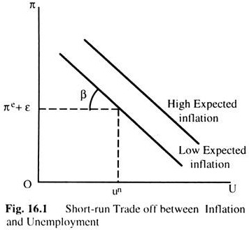
Fig. 16.1 shows the short-run trade-off between inflation and unemployment implied by the Phillips curve. The policymaker can manipulate AD to choose a combination of unemployment and inflation on this curve, called the short- run Phillips curve.

Notice that, the short-run Phillips curve depends on expected inflation. If expected inflation rises, the curve shifts upward, and the policymaker’s trade­off becomes less favourable: inflation is higher for any level of unemployment. The curve is higher when expected inflation is higher. Because people adjust their expectations of inflation over time, this tradeoff between inflation and unemployment holds only in the short-run.

Rational Expectations and Inflation:

Because the expectation of inflation influences the short-run trade-off between inflation and unemployment, a crucial question is how people form expectations. Thus far, we have been assuming that expected inflation depends on recently observed inflation. This adaptive expectation is too simplistic to be applicable in all circumstances.

Rational expectations assume that people optimally use all the available information, including information about current policies, to forecast the future. Because monetary and fiscal policies influence inflation, expected inflation also depends on the monetary and fiscal policies.

According to rational expectations theory, a change in monetary or fiscal policy will change expectations, and an evaluation of any policy change must incorporate this effect on expectations. This approach implies that inflation is less inertial than it first appears.

The advocates of rational expectations argue that the SRPC does not accurately represent the options available. They believe that if the policymakers are committed to reduce inflation, rational people will understand their com­mitment and reduce their expectations of inflation.

We can imagine that a painless disinflation, reducing inflation without causing recession, has two requirements. First, the plan to reduce inflation must be announced before the firms and workers who set wages and prices have formed their expectations. Second, the firms and workers must believe the announcement; otherwise, they will not revise their expectations of inflation.

If these requirements are met, the announcement will immediately shift the short-run trade-off between inflation and unemployment downward, permitting a lower rate of inflation without higher unemployment.

Although the rational expectations theory remains controversial, there is general agreement among economists that expectations of inflation influence the short-run trade-off between inflation and unemployment. Now we discuss how expectations influence inflation.

Inflation, Unemployment and the Phillips Curve:

Two goals of economic policymakers are low inflation and low unemployment. Inflation is a situation of continuously rising prices, where there must be continuous exogenous changes either in AD or AS. We first examine possible explanations of inflation within the framework of the comparative static model presented previously.

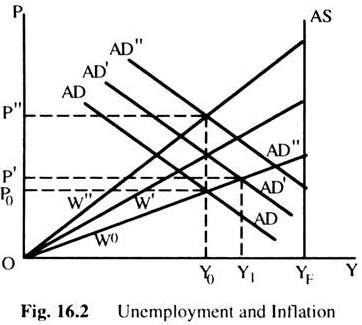
We then move on to examine a relationship between inflation and unemployment called the Phillips curve. In Fig. 16.2 we start with an equilibrium of less than full employment arising from a fixed money wage W₀. The equilibrium price level and real income are P₀ and Y₀, respectively, and there are some level of unemployment associated with that real income. Assume now that the government has a policy of maintaining ‘full employment’.

To achieve this goal the government carried out expansionary fiscal or monetary policy. This is shown by the shift of the AD curve to AD’. If this was the end of the story, the result of the government policy would be to raise the price level to P’, real income to Y’ and to lower unemployment by some amount. However, given the fixed money wage and the rise in prices as a result of the government policy, there is a fall in real wage.

Now the question is: What will happen if workers wish to maintain their real wage? To do that, they raise the money wage to W’. The effect of this is to raise the price level to P”, income to Y₀ and unemployment at their previous level. Thus, the efforts to maintain the real wage have resulted in a rise of the money wage and the price level, with no effect whatsoever on employment or real income.

What will happen if the government continues to maintain its ‘full employment’ policy and workers try to continue in their attempt to maintain their real wage? The AD curve will shift to AD” and money wage to W”, again leaving employment, real income and the real wage unchanged, but raising the money wage and the price level.

It may not take place immediately. There may be lags in the adjustment process. Thus, unemployment may fall for some time, and so the government policy may appear ‘successful’ until the adjustment in money wage—which may again raise the problem of excessive unemployment.

Let us take this analysis a little further. Assume that the process described above has continued for some time and people began to expect that prices will go on rising in the future. We also assume economy is at Y₀, P₀ and W₀ in Fig. 16.2. Now, suppose, the government undertakes an expansionary policy shown by the shift in the AD curve to AD’ and the price level rises to P’. Now to compensate for the expected rise in prices in the future, the money wage rate is raised to W”.

The adjustment in the money wage rate— to maintain real wage—is made on the basis of the expected price level rather than the current price level. In terms of the current price level this adjustment over-compensates for the rise in prices, so the real wage rises and income and employment fall. Now the government will have to undertake an expan­sionary policy just to maintain the original income Y₀. To increase income above Y₀ it would require an expansionary policy than before, and the effect on money wages and prices would be greater still.

In the above discussion the increases in AD occurred because of the ex­pansionary government policy to raise income and employment. But any continuous increase in AD could have similar effect. For example, if an inflation starts in the rest of the world and our country is initially in equilibrium at P₀, Y₀ and W⁰ as in Fig. 16.3, which has fixed exchange rate with the rest of the world, there will be an increase in exports, a decrease in imports and, thus, an increase in AD.

This will lead to a rise in prices, income and employment and a fall in real wage. If the money wage is raised to maintain the real wage, prices will rise even further. Whether this process would continue depends on the rate of inflation in the rest of the world relative to the home economy.

The above examples bring out some of the major themes in most current discussion of inflation; expansionary government policy to achieve certain goals, leading to a rise in prices, adjustment to the rise in prices and to the expected rise in prices: and the idea of importing inflation from abroad. Now the question is: Why do wages rise even though there is unemployment? What determines the formation of expectations? How fast do people adjust their expectation?

The first step to approach these questions is to pay more attention to the labour market than we have done so far. We have seen two possibilities in the labour market. In a flexible money wage, there is an unique full-employment equilibrium; in a rigid money wage, there would be some unemployment, depending on the money wage and the price level.

In a world in which information, acquiring skills, and mobility were costless, the assumption of flexible money wages would lead to full-employment and no involuntary unemployment, i.e. anybody wanting to work at the going wage rate could do so. What happens if all these costs are not zero? Now we would find that, there is always some unemployment in a changing economy.

It takes time to find the right job at the right wage; changing patterns of demand for goods in a changing technology require changing demands for particular skills, and it takes time to learn new skills. It is also costly to move and, therefore, sometimes worthwhile to wait in the expectation that mobility may not be necessary. All the above imply that the concept of full-employment is a very ambiguous one, and not a very sensible one, if taken literally to mean that no one is unemployed.

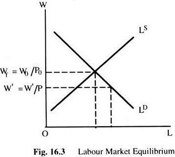
In Fig. 16.3 we represent the labour markets with a demand and supply of labour as a function of real wages, which is measured by a money wage divided by a price level, which, for the moment we assume given. Assume we have flexible money wages. At the real wage w_f = W₀/P₀ we have full employment in the sense that there is no excess demand or supply of labour. However, this does not mean that there is no unemployment.

Let us assume that, for a given structure of the labour market, unemployment is u_f as in Fig. 16.4. If the real wage is W’ = W’/P₀; what will happen? Because there is excess demand for labour, two things may happen. First, that the level of unemployment at this real wage is less than u_f. Second, that because of the excess demand the money wage will rise. The first proposition tells us that, if there is an excess demand for labour all the factors which led to unemployment at “full employment” would be mitigated.

With an excess demand for labour a wider range of skills would be demanded and the employer would be willing to substitute available skills for unavailable ones. It is also likely that capital would move to areas where labour is available, thus reducing the cost of labour mobility, and information may also spread more quickly. We shall thus assume that there is an indirect relationship between the excess demand for labour and unemployment.

Given the excess demand for labour, money wages will rise, until the equilibrium wage rate is reached. Let us also assume that the rate at which money wages rise depends on the excess demand for labour; the greater the pressure in the labour market the faster is the rate of change of money wages.

We thus have two relationships: first, a relationship between the excess demand for labour and unemployment; second, a relationship between the excess demand for labour and the rate of change of money wages. Combining these two we get a relationship between unemployment and inflation.

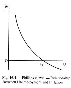
This relationship is shown in Fig. 16.4, where we measure on the vertical axis the percentage change in money wage rate per time period (W) and on the horizontal axis unemployment (u). The full-employment is represented by u_f, where there is no tendency for money wages to change, even though there is some unemployment which is known as natural rate of unemployment.

Any level of unemployment less than u_f implies that money wages will rise, because there is an excess demand for labour, and the rate at which they will rise depends on the excess demand for labour. At any unemployment greater than u_f there is an excess supply of labour and money wages are likely to fall, at a rate depending on the size of the excess supply.

The relationship shown in Fig. 16.4 is called the Phillips Curve — called after Prof. A. W. Phillips who first discovered the empirical relationship between the change in wages and employment in the U.K. between 1861-1957 with approximately the shape shown in the Fig. 16.4.

So far we have been discussing the relationship between the change in wages and unemployment. To relate the above discussion to an analysis of inflation we have to postulate some relationship between a change in money wages and a change in prices. There have been various ways in which this has been done, such as, mark up theories of pricing or marginal productivity theory of wage determination.

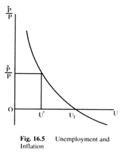
For our purpose it does not matter what is the exact relationship between the change in money wages and a change in prices. Let us assume that there is a positive relationship between the two. We can then translate Fig. 16.4 into Fig. 16.5, where we measure the rate of change of prices (P) on the vertical axis and unemployment on the horizontal axis.

Assume that the government wishes to maintain unemployment at u, less than u_f. To do that, the government has to induce a rate of price change of P’ which has been used in policy discussion to argue that the government has a choice between the two goals—inflation and unemployment.

The govern­ment can have no inflation if it is willing to accept the level of unemployment of u_f. This is a more complex development of the first theme discussed above in terms of the comparative static model but it does not incorporate the second theme—expectations and adjustment to them.

Expectations and the Phillips Curve:

To discuss expectations in the analysis of the Phillips Curve, and to sketch briefly some of the recent developments in this field we start with the labour market again. The real wage depends on two factors, the money wage and the price level. When there is inflation both the money wage and the price level are changing and both are expected to change to some extent.

An individual selling his labour receives a money wage offer and he has to assess what is the real wage represented by this offer. To do this he has to think what the price level could be over the period for which he offered the money wage.

For example, if an individual is offered a money wage W₀, the expected real wage is W₀/P₀ if the expected price level is P₀ and W₀/P₁ if the expected price level is P₁. The actual real wage is W₀ divided by whatever the price level is expected.

We thus have a possibility that the actual real wage may be greater or smaller than the real wage expected by the suppliers of labour on which they base their decision about how much labour to supply. We shall call that wage the expected real wage, W^e = W^e/P^e, the expected real wage is equal to the expected money wage divided by the expected price level.

We shall be interested in the rate of change of the variables and thus. W^e is the expected change of percentage in real wages. From the definition of expected real wages, W^e = W^e – P^e………. (1). Equation (1) states that, the expected percentage change in real wages is equal to the expected percentage change in money wages minus the expected change in the price level.

Now, assume that the expected change in money wages is equal to the actual change-in money wages which is equal to the rate of inflation—the percentage change in prices. We are also assuming that there is an ongoing inflation in which prices and money wages change at the same rate.

With this assumption, we have W^e = P – P. By substituting this into equation (1) we have W^e = P— P^e……. (2). Equation (2) says that the expected change in the real wage depends on the difference between the actual rate of inflation and the expected rate of inflation.

If the actual rate of inflation is greater than the expected rate, the expected real wage is increasing; if the actual inflation is equal to expected inflation, the expected real wage remains unchanged; and if the actual rate of inflation is less than the expected rate, the expected real wage is falling.

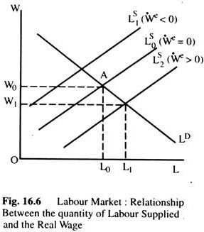
Fig. 16.6 shows the labour market. The supply curve shows the relationship between the quantity of labour supplied and the real wage. However, what is now important for the supply of labour is not the current real wage, but the expected real wage. Only if the expected change in the real wage is zero, is the current real wage the correct variable for the supply of labour. This is shown by the middle supply curve of labour where the expected rate of inflation is equal to the actual rate of inflation.

If the expected change in real wage is less, then, for each current real wage, labour supply would be reduced, because the current real wage is greater than the real wage as perceived by the suppliers of labour as shown by L^S₁(w^e <0) supply curve shifts to the left of L^s₀ line.

Again, from equation (2), this is the supply curve for which the expected rate of inflation is greater than the actual rate. Similarly, the supply curve L^s₂ (w^e > 0) shows a situation for which the expected change in the real wage is positive, which will occur if the expected rate of inflation is less than the actual rate.

Consider now that an initial equilibrium in which the actual inflation rate is equal to the expected inflation rate and assume that both are zero (no inflation). The equilibrium in the labour market is at A where real wage is W₀ and employment is L₀. Associated with this full-employment there is some level of unemployment u_f, which is called the natural rate of unemployment.

Assume that, now prices start rising, but at this level expectations about changes in the price level remain unchanged. Thus, the expected change in the price level is less than the actual change in the price level. The supply curve of labour moves to the right where real wage falls but the quantity of labour supplied rises to L₁ and unemployment falls.

The greater is the rise in prices, the larger is the difference between the actual change in prices and the expected change in prices. The shift of the supply curve to the right is greater, employment is larger and unemployment is smaller.

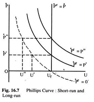
Let us translate this into a Phillips curve. Fig. 16.7 measures the rate of change of prices on the vertical axis and unemployment on the horizontal axis. When the rate of change in prices is zero—and everyone expects it to continue to be zero—equilibrium in the labour market in Fig. 16.6 is at W₀. L₀ with unemployment at u_f in Fig. 16.7. Assume that, now prices start rising at the rate P’ though people still expect inflation to be at the old rate namely zero.

The workers receive higher money wages and mistakenly belief that’ they are receiving higher real wages. Labour market equilibrium in Fig. 16. 6 is now at W₁L₁. Employment is greater and unemployment is smaller at u’ on Fig. 16.7.

If the change in prices and money wages is higher, say, P” the shift in the supply curve would be greater and unemployment smaller at u”. Thus, we get the downward sloping Phillips curve. However, it is clear that this Phillips curve was derived on the assumption that the expected change in prices is zero.

Now assume that, people begin to expect that the inflation will continue at some positive rate and the difference between the actual rate and expected rate of inflation will decrease and the supply curve of labour in Fig 16 6 will start shifting back. Employment will start falling and unemployment rising In Fig. 16.7 this can be shown by a shift of the Phillips curve to the right.

Each of the Phillips curves in Fig. 16.7 is drawn for some specified expected rate of inflation. When that expected rate of inflation is equal to the actual rate of inflation, unemployment will be u_f. Thus, the vertical Phillips curve at u_f shows the relationship between inflation and unemployment when the expected rate of inflation is equal to the actual rate. Along this curve there is no relationship between the two, and unemployment cannot be changed by increasing the rate of inflation, which is known as the long-run Phillips curve.

The Phillips curve analysis which takes into account expectations gives some insight not only into the effect of inflation but also into the effects of reducing inflation. In Fig. 16.8 we assume that, there has been an ongoing inflation at the rate P” to which everyone has adjusted. Thus, we are on the said Phillips curve along which the expected rate of inflation is equal to P”.

Now assume that the rate of inflation is reduced to P’ People still expect the rate of inflation to remain at the higher level, so we move along the solid Phillips curve. Unemployment, thus, rise to u’. Only after expectations become adjusted to the lower inflation rate docs the Phillips curve starts shifting to the left, and unemployment starts falling.

When full adjustment occurs, unemployment will be back at u_f and we will be on the dashed Phillips curve. Thus, once expectations about inflation have been built into the system it may be quite costly to reduce the rate of inflation.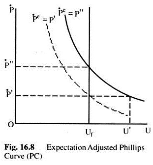

Inflation and Interest Rates:

Now we discuss the link between inflation and interest rates.

Two Interest Rates: Real and Nominal:

Economists call the interest rate that the bank pays for our deposits the nominal interest rate and the increase in our purchasing power the real interest rate. If i denotes the nominal interest rate, r the real interest rate, and π the rate of inflation, then the relationship among these three variables can be written as : r = i – π.

The real interest rate (r) is the difference between the nominal interest rate i and the rate of inflation.

The Fisher Effect:

We can show that the nominal interest rate is the sum of the real interest rate and the inflation rate: i = r + π. This is called the Fisher Equation which shows that the nominal interest rate can change for two reasons: because the real interest rate changes or because the inflation rate changes.

The quantity theory shows that the rate of money growth determines the rate of inflation. The Fisher Equation tells us to add the real interest rate and the inflation rate to determine the nominal interest rate. Thus, the quantity theory and the Fisher Equation together tell us how money growth affects the nominal interest rate.

Two Real Interest Rates: Ex Ante and Ex Post:

The real interest rate the borrower and lender expect when loan is made, is called the ex ante real interest rate, and the real interest rate actually realised, is called the ex post real interest rate.

Although borrowers and lenders cannot predict future inflation with cer­tainly, they do have some expectation of the inflation rate. Let π denote actual future inflation and π^e the expectation of future inflation. The ex ante real interest is i – π^e, and the ex post real interest rate is i – π. The two rates differ when actual inflation π differs from expected inflation π^e.

How does this distinction between expected and actual inflation modify the Fisher effect? The nominal interest rate cannot adjust to actual inflation, because actual inflation is not known when the nominal interest rate is set. It can adjust to expected inflation only. The Fisher effect is more precisely written as: i = r + π^e.

The extant interest rate r is determined by equilibrium in the commodity market, whereas the nominal interest rate i moves with changes in expected inflation π^e.