Policy of Managed Flexibility of Exchange Rates | International Economics

The rigidly fixed exchange rate policy and freely flexible exchange rate policy are at the two extremes. Either of the two extreme policies suffered from certain defects or problems. In practice, the different countries have attempted to adopt such exchange rate policies that tend to combine a certain degree of inflexibility with a reasonable degree of flexibility. Such policies are known as the policies of managed flexibility or controlled floating.

Certain categories of managed flexibility are discussed below:

1. Adjustable Peg System:

Under the Bretton Woods System, the exchange rates of different currencies were pegged in terms of gold or the U.S. dollar at the rate of $ 35 per ounce of gold. The nations were allowed to change the par values of their currencies when faced with a ‘fundamental’ disequilibrium.

In other words, the Bretton Woods System was originally conceived as an adjustable peg system. An adjustable peg system requires the defining of par value with a specific permitted band of variations along with the stipulation that the par value will be changed periodically and the currency devalued to correct a BOP deficit or revalued to correct a surplus.

Thus the adjustable peg policy involves the pegging of exchange at a given level at a given time. As the situation changes, the old peg (exchange parity), when it is no longer feasible, is abandoned and a new parity is established through devaluation or revaluation. In such a system, it is important that some specific objective rules are agreed upon and enforced to determine when a nation must readjust the par value and to what extent it should make the adjustment.

The working of adjustable peg system can be shown through Fig. 23.5.

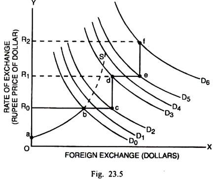
In Fig. 23.5, the foreign exchange (dollars) is measured along the horizontal scale. The rate of exchange (rupees price of dollar) is measured along the vertical scale. Given the demand for and supply curves D₀ and S respectively of foreign exchange, the original rate of exchange between dollar and rupee is R₀. This is the fixed or pegged exchange rate.

Even if the demand for foreign exchange increases and the demand curve shifts to D₁ and D₂, the rate of exchange remains pegged at the level R₀ and adjustment is made through the use of country’s exchange reserves. It means the supply curve, which had started from the point a rises positively upto point b and then becomes horizontal upto point c where the country exhausts its foreign exchange reserves.

If the demand curve shifts from D₂ to D₃, the country cannot maintain the old parity. Therefore, the exchange rate is adjusted at the higher level R₁. If the demand for foreign exchange increases and the demand curve shifts to D₄ and D₅, the same exchange parity R₁ is maintained again through the use of foreign exchange reserves. It means the supply curve, after moving vertically from c to d, moves horizontally upto e.

At this point the exchange reserves of the country have got exhausted. Further pegging at the level R₁ is not possible. The increase in demand, shown by the shift of demand curve from D₅ to D₆ must be adjusted now by pegging the exchange rate at a higher level R₂. In this system of adjustable peg, the effective supply curve of dollar has a zig-zag path a b c d e f and so on.

The adjustable peg system is sometimes also called as the system of maximum devaluation. A country faced with BOP deficit waits for some time and maintains the old peg through the pegging operations. When the pegging is no longer possible, the old equilibrium rate or peg becomes non-feasible. Then the country has to undertake a sudden big dose of devaluation of home currency.

In this way, the system of adjustable peg combines certain degree of exchange rate flexibility with stability of exchange rate and attempts to lead the economy towards a more realistic exchange rate.

Criticism:

The system of adjustable peg is criticised on the following grounds:

Firstly, in the IMF adjustable peg system, no clear cut operational definition of ‘fundamental’ disequilibrium was given. It was referred only in broad and vague terms as a large actual or potential deficit or surplus persisting over a series of years.

Secondly, most of the countries often give priority to the domestic objectives like maximum employment and price stability. This system provides no alternative for adjustment in the short run, when the imbalance has to be corrected by the use of exchange reserves and/or borrowing. These corrective measures detract from the achievement of domestic goals under this system.

It is only after a long period that the exchange rates have to be changed to restore equilibrium. In this context, Meade says that, “the stress on the present adjustable peg system has come to be put on the fixity of the peg rather than its adjustment.”

Thirdly, the deficit and surplus countries both are often reluctant to change the exchange rate for protecting their economic interests, for the reasons of prestige or to fend against the destabilising speculation. They will change the par value only when they are practically forced to do so.

Fourthly, the adjustable peg system causes a large scale destabilising speculation. If a country is faced with persistent deficit, the speculators can easily anticipate the extent by which the currency will be devalued. Accordingly, they start transferring funds out of a weak currency into stronger one with a view to avoid capital losses. Such speculation has adverse effects upon a relatively weak currency.

Fifthly, the IMF fixed parity or adjustable peg collapsed in 1973. Earlier, the U.S. dollar was the strongest currency. Most of the other countries wanted to build their exchange reserves in terms of dollars. This brought dollar under tremendous strain. This ultimately led the United States to disallow the convertibility of dollar into gold. It amounted to a collapse of IMF exchange system.

Sixthly, the system of adjustable peg involved a serious flaw in the form of IMF insistence upon the expenditure-reduction policies for correcting the BOP disequilibrium. It was not welcome to many countries which were inclined to follow the expenditure-raising policy for achieving higher growth rate and maximum welfare. Many of the countries adopted the expenditure-switching policies. That was also not acceptable to the IMF.

Seventhly, since under the adjustable peg system, the countries make change in exchange parity only when they have no other alternative or when they are forced to do so, it remains virtually a fixed exchange system.

Eighthly, in the opinion of Milton Friedman, “…this system can neither ensure sensitive, gradual and continuing adjustments in the rates of exchange, nor can it provide permanent stability in expectations. Therefore, it is clearly the worst of two worlds.”

2. Crawling Peg System:

The crawling peg system was popularised in mid-sixties by such prominent economists as William Fellner, J.H. Williamson, J. Black, J.E. Meade and C.J. Murphy. This system is a compromise between the extremes of freely fluctuating exchange rates and perfectly stable exchange rates. It was devised in order to avoid the disadvantage of relatively large changes in par values and possibly destabilising speculation associated with the system of adjustable peg.

In case of the Bretton Woods adjustable peg, sudden and large changes in exchange rates have to be made. These are clearly undesirable and should be avoided.

In addition, the authorities wait for a long time until the reserves of foreign exchange get exhausted. In case of crawling peg system, the par values are changed by small pronounced amounts or percentages at frequent and clearly specified intervals, such as one month or even a fortnight, until the equilibrium exchange rate is reached.

The extent of devaluation in this exchange system, undertaken by a country per specified period, is so small that it is not likely to cause destabilising speculation. Any possibility of destabilising speculation under the system of crawling peg can be offset by manipulating short-term interest rates.

This exchange rate policy known also as ‘trotting peg’ or ‘gliding parity” can be explained through Fig. 23.6.

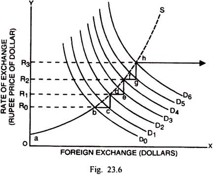
In Fig. 23.6, given demand and supply functions of foreign exchange (dollars) D₀ and S respectively, the original equilibrium rate of exchange is R₀. As there is an increase in the demand for foreign exchange, the demand function shifts to D₁.

Between b and c, the exchange rate R₀ is maintained through sale of dollars by the government. As the demand function further shifts to D₂, the devaluation in a small measure is undertaken. Between c and d, there is an adjustment to a new peg at R₁.

Between d and e, the government again supports exchange rate at R₁ by reducing its foreign exchange reserves. As the demand function further shifts from D₃ to D₄, the adjustment is again effected between e and f through another small measure of devaluation. If the demand function further shifts to D₅, the exchange parity R₂ is maintained again by the pegging operation (sale of dollars) for a short while between f and g.

When the demand curve shifts further to D₆, there is adjustment between point g and h again through a small dose of devaluation. The effective supply curve of dollar moves above the small ladder indicated by the path a b c d e f g h and so on.

Unlike the adjustable peg, which involves large but infrequent devaluations, there is a series of devaluations in small measures in the case of crawling peg. Under the adjustable peg system, the authorities wait for too long a period for making exchange adjustment until the bottom of the barrel of foreign exchange reserves of the country is broken.

In contrast, there are movements from one parity to another over a short period and there is no prolonged waiting until all the foreign reserves of the country are exhausted at one given rate of exchange.

While the adjustable peg system is closer to fixed exchange rate policy, the crawling peg system is closer to the flexible exchange rate policy. The crawling peg system can achieve even greater flexibility, if it is combined with wide bands of fluctuations. Earlier the IMF had permitted the exchange rate to fluctuate within a margin of 1 percent on either side of the exchange parity.

In December 1971 the IMF permitted that foreign exchange could fluctuate within a margin of 2.25 percent on either side of the exchange parity. This amendment imparted greater degree of flexibility to the exchange rates.

The crawling peg exchange rate policy is, indeed, superior to the policy of adjustable peg. The countries that want to use this system must, however, decide the frequency and the amount of change in their par values and the width of the band permitted for variations in exchange rate.

A crawling peg policy seems best suited for a developing country that faces real shocks and differential inflation rates. By December 1984, the system had been adopted in countries like Portugal, Brazil, Chile, Colombia and Madagascar and it seems to be functioning fairly well in these countries.

3. Policy of Managed Floating:

The exchange rates may continue to fluctuate, even if speculation is stabilising, on account of the variations that take place in the real sectors of the economy. The fluctuations in exchange rate tend to have an adverse effect upon the flow of international trade and investments. The Smithsonian Agreement made on December 18, 1971 provided for the widening of margin of fluctuations from 1 percent on each side of the exchange parity to 2.25 percent on each side of the par value of exchange.

European Snake:

The Werner Report of 1972, led to the institution of a scheme intended to reduce the fluctuations in the currencies of the members of the EC. The scheme required that the members restrict fluctuation between their currencies to ± 1.125 percent of their par values, but subject to the constraint that each would be allowed to fluctuate against the U.S. dollar by the full ± 2.25 percent allowed by the Smithsonian Agreement. This scheme was known as the ‘snake in the tunnel’. The ‘tunnel’ was later abandoned, when the member countries decided to float their currencies against the dollar.

The Smithsonian Agreement broke down following the U.S. devaluation of dollar on February 32, 1973. Several countries including Britain, Canada, Japan, Switzerland, India and some smaller countries had floating exchange rates in March 1973. The countries of EC continued to have a “joint float” even after March 1973. Since the EC currencies could fluctuate relative to other currencies irrespective of any fixed margin or band, the exchange rate policy of EC countries was likened to a “snake in the lake.”

The Jamaica Agreement of January 1976 formalised the regime of floating exchange rates under the auspices of the IMF. A majority of the member countries of the IMF were forced to float their currencies on account of several developments in the 1970’s such as large scale short-term capital movements, failure of central banks to prevent speculation in currencies, the oil crisis, inflation, industrial recession in the advanced countries and severe pressure on the U.S. dollar.

Several currencies were floated in the foreign exchange market so that they should assume their natural value (or rate of exchange) relative to dollar or a basket of principal currencies. By 1978, the system of floating exchange rates had come to stay.

The system of floating exchange rates was not, in fact, a system of freely flexible exchange rates but of a managed float. Under a system of managed floating exchange rate, the monetary authorities of the different countries are entrusted with the responsibility to intervene in foreign exchange markets to smoothen out these short run fluctuations without attempting to affect the long- term trend in exchange rates. To the extent the countries are successful in this endeavor; they can secure the benefits that result from fixed exchange rates.

At the same time, they retain the flexibility in adjusting the BOP disequilibria. It is true that the monetary authorities are in no better position than traders, investors or professional speculators to know what the long-term trend in foreign exchange rate is. Such knowledge is not even required to stabilise the short run fluctuations in exchange rates, when a country has adopted a policy of “leaning against the wind.”

In case of this policy, the central banks intervene only to moderate the short run fluctuations through using (to a limited extent) or absorbing the international exchange reserves. Such a policy reduces the short run fluctuations in the exchange rate without affecting the long term trend in exchange rates. It implies that even under a policy of managed float there is need of maintaining some amount of foreign exchange reserves.

Clean and Dirty Float Systems:

In connection with a system of managed float, it may be pointed out that a distinction is sometimes made between a clean float and dirty float.

(i) Clean Float:

In case of clean float, the rate of exchange is allowed to be determined by the free market forces of demand and supply of foreign exchange. The exchange rate is permitted to move up and down. The foreign exchange market itself corrects the excess demand or excess supply conditions without the intervention of monetary authority. Thus, the policy of clean float is identical to the policy of freely fluctuating exchange rates.

(ii) Dirty Float:

In case of a dirty float, the exchange rate is sought to be determined by the market forces of demand and supply for foreign exchange. However, the monetary authority intervenes in the foreign exchange market through the pegging operations either to smoothen or to eliminate the fluctuations altogether. It means even the long term trend in exchange rate is manipulated by the monetary authority. Such a policy of managed float is understood as the policy of ‘dirty float’. The clean float and dirty float are distinguished through Fig. 23.7.

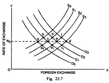
Initially, given the demand and supply functions of foreign exchange as D₀ and S₀ respectively, the equilibrium rate of exchange R₀ is determined at point a. Under the alternate pressures of BOP deficits and surpluses, the demand and supply curves undergo shifts. The policy of clean float causes the equilibrium rate of exchange to move along the path ab₁cd₁ef₁g.

Alternatively, under the free adjustment without central banking intervention, the exchange rate, in case of clean float, moves along the path a b c d e f g. In these two cases of clean float, the exchange rate is fairly stable around the level R₀.

On the opposite, when there is a policy of dirty float and the central bank is prepared to intervene through the sale or purchase of foreign exchange and the variations in exchange rate are not allowed to take place. The movement takes place directly from a to c, then from c to e and again from e to g.

The clean float policy ensures the exchange rate stability with a certain degree of flexibility. The dirty float, on the opposite, does not permit flexibility in the exchange rate.

The policy of dirty float does not necessarily mean that there will be complete rigidity of the rate of exchange. The essential point is the intervention of the monetary authority to effect the exchange rate variations in a way which will favour the home country, no matter how the foreign country will be affected.

For instance, a country might be tempted to intervene in the exchange market in such a way as to keep the exchange rate high (i.e., the home currency is retained at a depreciated level) to stimulate its exports. It is a beggar-my-neigbour policy and is likely to provoke retaliation.

A dirty float results not only in deliberate manipulations of exchange rate, it also affects the long term trend of fluctuations. The distortions caused by the dirty float are clearly detrimental to the smooth flow of international trade and investment.

Despite the adoption of managed floating system by the world since 1973.the wide exchange rate variations have continued to take place. For instance, there was large appreciation of the U.S. dollar between 1980 and February 1985. It was followed by equally large depreciation of that currency. That clearly indicates that large exchange rate disequilibria can arise and persist over several years under the present managed floating.