Theory of Consumer Behaviour (Indifference-Curves)

Assumptions:

1. Rationality:

The consumer is assumed to be rational he aims at the maximization of his utility, given his income and market prices. It is assumed he has full knowledge (certainty) of all relevant information.

2. Utility is ordinal:

It is taken as axiomatically true that the consumer can rank his preferences (order the various ‘baskets of goods’) according to the satisfaction of each basket. He need not know precisely the amount of satisfaction. It suffices that he ex­presses his preference for the various bundles of commodities. It is not necessary to assume that utility is cardinally measurable. Only ordinal measurement is required.

3. Diminishing marginal rate of substitution:

Preferences are ranked in terms of in­difference curves, which are assumed to be convex to the origin. This implies that the slope of the indifference curves increases. The slope of the indifference curve is called the marginal rate of substitution of the commodities. The indifference-curve theory is based, thus, on the axiom of diminishing marginal rate of substitution.

4. The total utility of the consumer depends on the quantities of the commodities consumed

U = f (q₁, q₂,…, q_x, q_y,………….. q_n)

5. Consistency and transitivity of choice:

It is assumed that the consumer is consistent in his choice, that is, if in one period he chooses bundle A over B, he will not choose B over A in another period if both bundles are available to him.

The consistency assump­tion may be symbolically written as follows:

If A > B, then B !> A

Similarly, it is assumed that consumer’s choices are characterised by transitivity: if bundle A is preferred to B, and B is preferred to C, then bundle A, is preferred to C.

Symbolically we may write the transitivity assumption as follows:

If A > B, and B > C, then A > C

Equilibrium of the consumer:

To define the equilibrium of the consumer (that is, his choice of the bundle that maximizes his utility) we must introduce the concept of indifference curves and of their slope (the marginal rate of substitution), and the concept of the budget line. These are the basic tools of the indifference curves approach.

Indifference curves:

An indifference curve is the locus of points – particular combinations or bundles of goods-which yield the same utility (level of satisfaction) to the consumer, so that he is indifferent as to the particular combination he consumes.

An indifference map shows all the indifference curves which rank the preferences of the consumer. Combinations of goods situated on an indifference curve yield the same utility. Combinations of goods lying on a higher indifference curve yield higher level of satisfaction and are preferred. Combinations of goods on a lower indifference curve yield a lower utility.

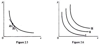
An indifference curve is shown in figure 2.5 and a partial indifference map is depicted in figure 2.6. It is assumed that the commodities y and x can substitute one another to a certain extent but are not perfect substitutes.

The negative of the slope of an indifference curve at any one point is called the marginal rate of substitu­tion of the two commodities, x and y, and is given by the slope of the tangent at that point

[Slope of indifference curve] = – dy/dx = MRS_x,y

The marginal rate of substitution of x for y is defined as the number of units of commodity y that must be given up in exchange for an extra unit of commodity x so that the con­sumer maintains the same level of satisfaction. With this definition the proponents of the indifference-curves approach thought that they could avoid the non-operational concept of marginal utility.

In fact, what they avoid is the assumption of diminishing individual marginal utilities and the need for their measurement. The concept of marginal utility is implicit in the definition of the MRS, since it can be proved that the marginal rate of substitution (the slope of the indifference curve) is equal to the ratio of the marginal utilities of the commodities involved in the utility function

MRS_x,y = MU_x / MU_y or MRS_y,x = MU_y/Mu_x

Furthermore, the indifference-curves theorists substitute the assumption of diminishing marginal utility with another which may also be questioned, namely the assumption that the indifference curves are convex to the origin, which implies diminishing MRS of the commodities.

Properties of the indifference curves:

1. An indifference curve has a negative slope, which denotes that if the quantity of one commodity (y) decreases, the quantity of the other (x) must increase, if the consumer is to stay on the same level of satisfaction.

2. The further away from the origin an indifference curve lies, the higher the level of utility it denotes bundles of goods on a higher indifference curve are preferred by the rational consumer.

3. Indifference curves do not intersect. If they did, the point of their intersection would imply two different levels of satisfaction, which is impossible.

Proof:

The slope of a curve at any one point is measured by the slope of the tangent at that point. The equation-of a tangent is given by the total derivative or total differential, which shows the total change of the function as all its determinants change.

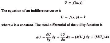
The total utility function in the case of two commodities x and y is

It shows the total change in utility as the quantities of both commodities change. The total change in U caused by changes in y and x is (approximately) equal to the change in y multiplied by its marginal utility, plus the change in x multiplied by its marginal utility.

Along any particular indifference curve the total differential is by definition equal to zero. Thus for any indifference curve

4. The indifference curves are convex to the origin. This implies that the slope of an indifference curve decreases (in absolute terms) as we move along the curve from the left downwards to the right: the marginal rate of substitution of the commodities is diminishing. This axiom is derived from introspection, like the ‘law of diminishing marginal utility’ of the cardinalist school.

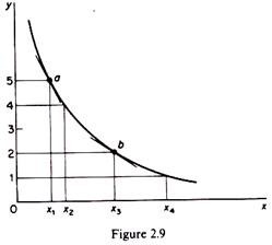
The axiom of decreasing marginal rate of substitution expresses the observed behavioural rule that the number of units of x the consumer is willing to sacrifice in order to obtain an additional unit of y increases as the quantity of y decreases. It becomes increasingly difficult to substitute x for y as we move along the indifference curve. In figure 2.9 the fifth unit of y can be substituted for x by the consumer giving up x₁ x₂ of x; but to substitute the second unit of y and still retain the same satisfaction the consumer must give up a much greater quantity of x, namely x₃ x₄.

The budget constraint of the consumer:

The consumer has a given income which sets limits to his maximizing behaviour. Income acts as a constraint in the attempt for maximizing utility. The income constraint, in the case of two commodities, may be written

Y=P_xq_x + P_yq_y (2.1)

We may present the income constraint graphically by the budget line, whose equation is derived from expression 2.1, by solving for q_y

q_y = 1 / P_y Y – p_x / p_y q_x

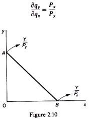
Assigning successive values to q_x (given the income, Y and the commodity prices, P_x, P_y), we may find the corresponding values of q_y. Thus, if q_x = 0 (that is, if the con­sumer spends all his income on y) the consumer can buy Y/P_y units of y. Similarly, if q_y = 0 (that is, if the consumer spends all his income on x) the consumer can buy Y/P_x units of x. In figure 2.10 these results are shown by points A and B. If we join these points

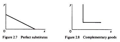
This assumption implies that the commodities can substitute one another, but are not perfect substitutes. If the commodities are perfect substitutes the indifference curve becomes a straight line with negative slope (figure 2.7). If the commodities are complements the indifference curve takes the shape of a right angle (figure 2.8).

In the first case the equilibrium of the consumer may be a corner solution, that is, a situation in which the consumer spends all his income on one commodity. This is sometimes called ‘monomania’. Situations of ‘monomania’ are not observed in the real world and are usually ruled out from the analysis of the behaviour of the consumer. In the case of complementary goods, indifference-curves analysis breaks down, since there is no possibility of substitution between the commodities.

with a line we obtain the budget line, whose slope is the ratio of the prices of the two commodities. Geometrically the slope of the budget line is

OA / OB = Y / P_y / Y / P_x = P_x / P_y

Mathematically the slope of the budget line is the derivative

Derivation of the equilibrium of the consumer:

The consumer is in equilibrium when he maximizes his utility, given his income and the market prices. Two conditions must be fulfilled for the consumer to be in equilibrium.

The first condition is that the marginal rate of substitution be equal to the ratio of commodity prices

MRS_{x, y} = MU_x / MU_y = P_x / P_y

This is a necessary but not sufficient condition for equilibrium. The second condition is that the indifference curves be convex to the origin. This condition is fulfilled by the axiom of diminishing MRS_{x, y}, which states that the slope of the indifference curve decreases (in absolute terms) as we move along the curve from the left downwards to the right.

Graphical presentation of the equilibrium of the consumer:

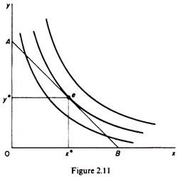
Given the indifference map of the consumer and his budget line, the equilibrium is defined by the point of tangency of the budget line with the highest possible indifference curve (point e in figure 2.11).

At the point of tangency the slopes of the budget line (P_x/P_y) and of the indifference curve (MRS_{x, y} = MU_x/MU_y) are equal:

MU_X = MU_y = P_X / P_y

Thus the first-order condition is denoted graphically by the point of tangency of the two relevant curves. The second-order condition is implied by the convex shape of the indifference curves. The consumer maximizes his utility by buying x and y of the two commodities.

Mathematical derivation of the equilibrium:

Given the market prices and his income, the consumer aims at the maximization of his utility. Assume that there are n commodities available to the consumer, with given market prices P₁, P₂, .., P_n. The consumer has a money income (V), which he spends on the available commodities.

Formally the problem may be stated as follows:

We use the ‘Lagrangian multipliers’ method for the solution of this constrained maximum. The steps involved in this method may be outlined as follows:

(a) Rewrite the constraint in the form

(q₁P₁ + q₂P₂ + . . . + q_n P_n – Y) = 0

(b) Multiply the constraint by a constant A, which is the Lagrangian multiplier

λ (q₁P₁ + q₂P₂ + . . . + q_n P_n – Y) = 0

(c) Subtract the above constraint from the utility function and obtain the ‘composite function’

ɸ = U – λ (q₁P₁ + q₂P₂ + . . . + q_n P_n – Y) = 0

It can be shown that maximization of the ‘composite’ function implies maximization of the utility function.

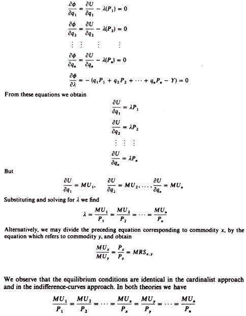
The first condition for the maximization of a function is that its partial derivatives be equal to zero. Differentiating ɸ with respect to q₁, …, q_n and λ, and equating to zero we find

Thus, although in the indifference-curves approach cardinality of utility is not required, the MRS requires knowledge of the ratio of the marginal utilities, given that the first- order condition for any two commodities may be written as

MU_x / MU_y = P_x / P_y = MRS _x,y

Hence the concept of marginal utility is implicit in the definition of the slope of the indifference curves, although its measurement is not required by this approach. What is needed is a diminishing marginal rate of substitution, which of course does not require diminishing marginal utilities of the commodities involved in the utility function.

Derivation of the demand curve using the indifference-curves approach:

Graphical derivation of the demand curve:

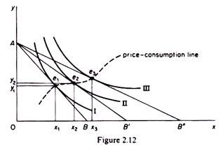
As the price of a commodity, for example of x, falls, the budget line of the consumer shifts to the right, from its initial position (AB) to a new position (AB) due to the increase in the purchasing power of the given money income of the consumer. With more purchasing power in his possession the consumer can buy more of x (and more of y). The new budget line is tangent to a higher indifference curve (e.g. curve II). The new equilibrium occurs to the right of the original equilibrium (for normal goods) showing that as price falls more of the commodity will be bought.

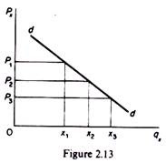
If we allow the price of x to fall continuously and we join the points of tangency of succes­sive budget lines and higher indifference curves we form the so-called price-consumption line (figure 2.12), from which we derive the demand curve for commodity x. At point e₁ the consumer buys quantity x₁ at price y₁. At point e₂ the price, y₂, is lower than y₁, and the quantity demanded has increased to x₂, and so on. We may plot the price- quantity pairs defined by the points of equilibrium (on the price-consumption line) to obtain a demand curve, as shown in figure 2.13.

The demand curve for normal commodities will always have a negative slope, denoting the ‘law of demand,’ (the quantity bought increases as the price falls). In the indifference-curves approach the ‘law of demand’ is derived from what is known as Slutsky’s theorem, which states that the substitution effect of a price change is always negative (relative to the price if the price increases, the quantity demanded decreases and vice versa). The formal proof of Slutsky’s theorem involves sophisticated math­ematics. However, we may show graphically the implications of this theorem.

We saw that a fall in the price of x from P₁ to P₂ resulted in an increase in the quantity demanded from x₁ to x₂. This is the total price effect which may be split into two separate effects, a substitution effect and an income effect. The substitution effect is the increase in the quantity bought as the price of the commodity falls, after ‘adjusting’ income so as to keep the real purchasing power of the consumer the same as before.

This adjustment in income is called compensating variation and is shown graphically by a parallel shift of the new budget line until it becomes tangent to the initial indifference curve (figure 2.14). The purpose of the compensating variation is to allow the consumer to remain on the same level of satisfaction as before the price change. The compensated-budget line’ will be tangent to the original indifference curve (I) at a point (e’₁) to the right of the original tangency (e₁), because this line is parallel to the new budget line which is less steep than the original one when the price of x falls. The movement from point e₁ to e’₁ shows the substitution effect of the price change the consumer buys more of x now that it is cheaper, substituting y for x.

However, the compensating variation is a device which enables the isolation of the substitution effect, but does not show the new equilibrium of the consumer. This is defined by point e₂ on the higher indiffer­ence curve II. The consumer has in fact a higher purchasing power, and, if the commodity is normal, he will spend some of his increased real income on x, thus moving from x’₁ to x₂. This is the income effect of the price change.

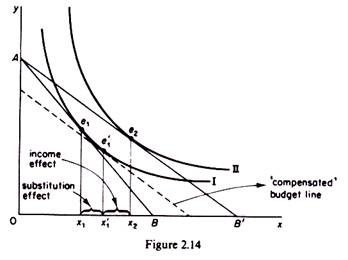
The income effect of a price change is negative for normal goods and it reinforces the negative substitu­tion effect (figure 2.14). If, however, the commodity is inferior, the income effect of the price change will be positive: as the purchasing power increases, less of x will be bought. Still for most of the inferior goods the negative substitution effect will more than offset the positive income effect, so that the total price effect will be negative. Thus the negative substitution effect is in most cases adequate for establishing the law of demand.

(It is when the income effect is positive and very strong that the ‘law of demand’ does not hold. This is the case of the Giffen goods, which are inferior and their demand curve has a positive slope. Giffen goods are very rare in practice.)

It should be noted that although Slutsky’s theorem can be proved mathematically, its proof is based on the axiomatic assumption of the convexity of the indifference curves.

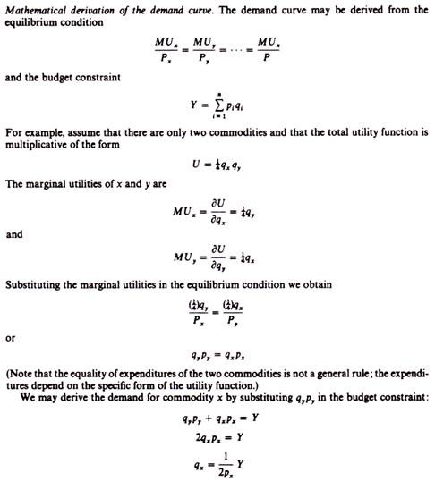
Thus the demand for x is negatively related to its own price p_x and positively to income Y.

Similarly the demand for y is obtained by substituting q_xp_x in the budget constraint

qy = 1 / 2p_y Y

In our particular example the demand curves are symmetric due to the particular multiplicative form of the consumer’s utility function which we assumed.

Critique of the indifference-curves approach:

The indifference-curves analysis has been a major advance in the field of consumer’s demand. The assumptions of this theory are less stringent than for the cardinal utility approach. Only ordinality of preferences is required, and the assumption of constant utility of money has been dropped.

The methodology of indifference curves has provided a framework for the measure­ment of the ‘consumer’s surplus’, which is important in welfare economics and in design­ing government policy.

Perhaps the most important theoretical contribution of this approach is the establish­ment of a better criterion for the classification of goods into substitutes and comple­ments. Earlier theorists were using the total effect of a price change for this purpose, without compensating for the change in real income. The classification was based on the sign of the cross-elasticity of demand

e_yx = ∂q_y / ∂p_x. p_x / q_y

Where the total change in the quantity of y was considered as a result of a change in the price of x. A positive sign of the cross-elasticity implies that x and y are substitutes; a negative sign implies that the commodities are complements. This approach may easily lead to absurd classifications if the change in the price of x is substantial.

For example, if the price of beef is halved it is almost certain that both the consumption of beef and of pork will be increased, due to the increase of the real income of the consumer. This would imply a negative cross-elasticity for pork, and hence pork would be classified as a complementary commodity to beef!

Hicks’ suggested measuring the cross-elasticity after compensating for changes in real income. Thus, according to Hicks, goods x and y are substitutes if, after com­pensating for the change in real income (arising from the change in the price of x) a decrease in the price of x leads to a decrease in the quantity demanded of y.

Although this criterion is theoretically more correct than the usual approach based on the total change in the quantity of y as a result of a change in the price of x, in practice its application is impossible because it requires knowledge of the individual preference functions, which cannot be statistically estimated. On the other hand, the usual approach of the total price effect is feasible because it requires knowledge of the market demand functions which can be empirically estimated.

Although the advantages of the indifference-curves approach are important, the theory has indeed its own severe limitations. The main weakness of this theory is its axio­matic assumption of the existence and the convexity of the indifference curves. The theory does not establish either the existence or the shape of the indifference curves. It assumes that they exist and have the required shape of convexity.

Furthermore, it is questionable whether the consumer is able to order his preferences as precisely and rationally as the theory implies. Also the preferences of the consumers change con­tinuously under the influence of various factors, so that any ordering of these preferences, even if possible, should be considered as valid for the very short run. Finally, this theory has retained most of the weaknesses of the cardinalist school with the strong assumption of rationality and the concept of the marginal utility implicit in the definition of the marginal rate of substitution.

Another defect of the indifference curves approach is that it does not analyze the effects of advertising, of past behaviour (habit persistence), of stocks, of the inter­dependence of the preferences of the consumers, which lead to behaviour that would be considered as irrational, and hence is ruled out by the theory. Furthermore specula­tive demand and random behaviour are ruled outlet these factors are very important for the pricing and output decisions of the firm.