
Read this article to learn about the Theory of Consumer’s Behaviour Utility Analysis, Meaning of Utility, Marshall’s Cardinal Utility Analysis, Limitations of the Law of Equimarginal Utility, Critical Evaluation of Marshall’s Cardinal Utility Analysis.
Theory of Consumer’s Behaviour Utility Analysis
Contents:
- Introduction to the Theory of Consumer’s Behaviour Utility Analysis
- Meaning of Utility
- Marshall’s Cardinal Utility Analysis
- Limitations of the Law of Equimarginal Utility
- Critical Evaluation of Marshall’s Cardinal Utility Analysis
1. Introduction to the Theory of Consumer’s Behaviour Utility Analysis:
The price of a product depends upon the demand for and the supply of it. In this part of the article we are concerned with the theory of demand, which explains the demand for a good and the factors determining it. Individual’s demand for a product depends upon the price of the product, income of the individual, and the prices of related goods.
It can be stated in the following functional form:
ADVERTISEMENTS:
Dx = f(Px, I, Py, Pz etc.)
Where Dx stands for the demand for good X, Px for price of good X, I for individual’s income, Py, Pz etc., for the prices of related goods. But among these determinants of demand, economists single out price of the good in question as the most important factor governing the demand for it. Indeed, the function of a theory of demand is to establish a relationship between quantity demanded of a good and its price and to provide an explanation for it.
From time to time, different theories have been advanced to explain consumer’s demand for a good and to derive a valid demand theorem. Cardinal utility analysis is the oldest theory of demand which provides an explanation of consumer’s demand for a product and derives the law of demand which establishes an inverse relationship between price and quantity demanded of a product.
Recently, cardinal utility approach to the theory of demand has been subjected to server criticisms and as a result some alternative theories, namely, Indifference Curves Analysis, Samuelson’s Revealed Preference Theory, have been propounded. Through cardinal utility approach to the theory of demand is very old, its final shape emerged at the hands of Marshall. Therefore, it is Marshallian utility analysis of demand which has been discussed in this article.
2. The Meaning of Utility:
People demand goods because they satisfy the wants of the people. The utility means want-satisfying power of a commodity. It is also defined as property of the commodity which satisfies the wants of the consumers. Utility is a subjective thing and resides in the mind of men. Being subjective it varies with different persons, that is, different persons derive different amounts of utility from a given good. People know utility of goods by their psychological feeling.
ADVERTISEMENTS:
The desire for a commodity by a person depends upon the utility he expects to obtain from it. The greater the utility he expects from a commodity, the greater his desire for that commodity. It should be noted that no question of ethics or morality is involved in the use of the word ‘utility’ in economics.
The commodity may not be useful in the ordinary sense of the term even then it may provide utility to some people. For instance, alcohol may actually harm a person but it possesses utility for a person whose want it satisfies. Thus, the desire for alcohol may be considered immoral by some people but no such meaning is conveyed in the economic sense of the term. Thus, in economics the concept of utility is ethically neutral.
Total Utility and Marginal Utility:
It is important to distinguish between total utility and marginal utility. Total utility of a commodity to a consumer is the sum of utilities which he obtains from consuming a certain number of units of the commodity per period. Consider Table 5.1 where a utility of a consumer from cups of tea per day is given. If the consumer consumes one cup of tea per day, he gets utility equal to 12 utils.

On consuming two units of the commodity per day his utility from the two units of the commodity rises to 22 utils and so on. When he takes 6 cups of tea per day, his total utility, that is, total utility of all the 6 units taken per day goes up to 41 utils. Generally, the greater the number of units of a commodity consumed by an individual, the greater the total utility he gets from the commodity. Thus, total utility is the function of the quantity of the commodity consumed.
It should however be noted that as the units of a commodity increases, total utility increases at a diminishing rate. When want of the consumer for a particular commodity is fully satisfied by consuming a certain quantity of the commodity, further increases in consumption of the commodity will cause a decline in total utility of the consumer. The number of units of commodity consumed at which a consumer is fully satisfied is called satiation quantity.
Beyond the satiation point, total utility decreases if more is consumed. It will be seen from Table 5.1 that total utility declines when the consumer consumes more than 6 units of the commodity. This happens because beyond satiety point more consumption of a good actually harms the consumer which causes a decline in utility or satisfaction from the commodity.
Marginal Utility:
Marginal utility of a commodity to a consumer is the extra utility which he gets when he consumes one more unit of the commodity. In other words, marginal utility is the addition made to the total utility when one more unit of a commodity is consumed by an individual. The concept of marginal utility can be easily understood from Table 5.1.
When the consumer takes two cups of tea instead of one cup his total utility increases from 12 to 22 utils. This means that the consumption of the second unit of the commodity has made addition to the total utility by 10 utils. Thus marginal utility is here equal to 10 utils.
Further when the number of cups of tea consumed per day from 2 to 3, the total utility increases from 22 to 30 utils. That is, the third unit of tea has made an addition of 8 utils to the total utility. Thus 8 is the marginal utility of the third of consumption of tea. Beyond 6 cups of tea consumption per day, total utility declines and therefore marginal utility becomes negative.
Marginal utility can be expressed as under:
![]()
Where n is any given number?
ADVERTISEMENTS:
In terms of calculus, it can be expressed as:
![]() , where ΔQ = 1
, where ΔQ = 1
Therefore, in graphical analysis, marginal utility of a commodity can be known by measuring the slope of the total utility curve.
3. Marshall’s Cardinal Utility Analysis:
Assumptions of Marshall’s Cardinal Utility Analysis:
Marginal utility analysis of demand is based upon certain important assumptions. Before explaining how utility analysis explains consumer’s equilibrium in regard to the demand for goods, it is essential to describe those basic assumptions on which the whole cardinal utility analysis rests.
ADVERTISEMENTS:
The basic assumptions or premises of utility analysis are as follows:
1. The Cardinal Measurability of Utility:
The exponents of a cardinal utility theory or what is also called marginal utility analysis regards utility to be a cardinal concept. In other words, they hold that utility is a measurable and quantifiable entity. According to them, a person can express the utility or satisfaction he derives from the goods in the quantitative cardinal terms.
Thus, a person can say that he derives utility equal to 10 utils from the consumption of a unit of good A, and 20 utils from the consumption of a unit of good B. Moreover, the cardinal measurement of utility involves that a person can compare in respect of size, that is, how much one level of utility is greater than another.
ADVERTISEMENTS:
For example, a person can say whether the utility he gets from the consumption of one unit of good B is double the utility he obtains from the consumption of one unit of good A. Marshall argues that the amount of money which a person is prepared to pay for a unit of a good rather than go without it is a measure of the utility he derives from that good.
Thus, according to him, money is the measuring rod of utility. Some economists belonging to the cardinalist school measure utility in imaginary units called “utils”. They assume that a consumer is capable of saying that one apple provides him utility equal to 4 utils and one orange gives him utility equal to 2 utils. Further, on this ground, he can say that he gets twice as much utility from an apple as from an orange.
2. The Hypothesis of Independent Utilities:
The second important tenet of the cardinal utility analysis is the hypothesis of independent utilities. On this hypothesis, the utility which a consumer .derives from a good is the function of the quantity of that good and of that good only. In other words, the utility which a consumer obtains from a good does not depend upon the quantity consumed of other goods; it depends upon the quantity purchased of that good alone.
On this assumption, the total utility which a person gets from a collection of goods purchased by him is simply the total sum of the separate utilities of the goods. Thus, the cardinalist school regards utility as ‘additive’, that is, separate utilities of different goods can be added to obtain the total sum of the utilities of all goods purchased.
3. Constancy of the Marginal Utility of Money:
ADVERTISEMENTS:
Another important assumption of Marshall’s marginal utility analysis is the constancy of the marginal utility of money. Thus, while the cardinal utility analysis assumes that marginal utilities of commodities diminish as more of them are purchased or consumed, but the marginal utility of money remains constant throughout when the individual is spending money on a good and due to which the amount of money with him varies.
Marshall measured marginal utilities in terms of money. But measurement of marginal utility of goods in terms of money is only possible if the marginal utility of money itself remains constant. It should be noted that the assumption of constant marginal utility of money is very crucial to the Marshallian utility analysis, because otherwise Marshall could not measure the marginal utilities of goods in terms of money.
If the money which is the unit of measurement itself varies as one is measuring with it, it cannot then yield correct measurement of the marginal utility of the good.
Prof. Tapas Majumdar rightly says:
“If money is supposed to provide the measuring rod of utility, then evidently as with all measuring rods, its unit must be invariant it must measure the same amount of utility in all circumstances.”
When the price of a good falls and as a result real income of the consumer rises, the marginal utility of money to him will fall but Marshall ignored this and assumed that marginal utility of money did not change as a result of the change in price. Likewise, when the price of a good rises, the real income of the consumer will fall and his marginal utility of money will rise. But Marshall ignored this and assumed that marginal utility of money remains the same.
ADVERTISEMENTS:
Marshall defended this assumption on the ground that “his (the individual consumer’s) expenditure on any one thing … is only a small part of his whole expenditure.” Therefore, according to him, a change in price of a good does not have any significant effect on the real income of a consumer.
4. Introspective Method:
Another important hypothesis of the cardinal utility analysis is the use of introspective method for judging the behaviour of marginal utility. In the introspective method the economists reconstruct or built up with the help of their own psychological experience the trend of feeling which goes on in other men’s mind.
From his own response to certain forces and by psychological experience and observation one gains understanding of the way other people’s minds would work in similar situations. To sum up, in introspective method we attribute to another person what we know of our own mind. That is, by looking into ourselves we see inside the heads of other individuals.
So the law of diminishing marginal utility is based upon introspection. We know from our own mind that as we have more of a thing, the less utility we derive from an additional unit of it. We conclude from it that other individuals’ mind will work in a similar fashion, that is, marginal utility to them of a good will diminish as they have more units of it.
Law of Marshall’s Cardinal Utility:
With the above basic assumptions, the founders of cardinal utility analysis have developed two laws which occupy an important place in economic theory and have several applications and uses.
ADVERTISEMENTS:
These two laws are:
1. Law of Diminishing Marginal Utility, and
2. Law of Equimarginal Utility.
It is with the help of these two laws about consumers’ behaviour that the exponents of utility analysis have derived the law of demand. We explain below these two laws in detail.
1. Law of Diminishing Marginal Utility:
An important tenet of marginal utility analysis relates to the behaviour of marginal utility. This familiar behaviour of marginal utility has been stated in the Law of Diminishing Marginal Utility according to which marginal utility of a good diminishes as an individual consumes more units of the good.
ADVERTISEMENTS:
In other words, as a consumer takes more units of a good, the extra utility or satisfaction that he derives from an extra unit of the good goes on falling. It should be carefully noted that it is the marginal utility and not the total utility that declines with the increase in the consumption of a good. The law of diminishing marginal utility means that the total utility increases but at a decreasing rate.
Marshall who was the famous exponent of the marginal utility analysis has stated the law of diminishing marginal utility as follows:
“The additional benefit which a person derives from a given increase of his stock of a thing diminishes with every increase in the stock that he already has.”
This law is based upon two important facts. Firstly, while the total wants of a man are virtually unlimited, each single want is satiable. Therefore, as an individual consumes more and more units of a good, intensity of his want for the good goes on falling and a point is reached where the individual no longer wants any more units of the good.
That is, when saturation point is reached, marginal utility of a good becomes zero. Zero marginal utility of a good implies that the individual has all that he wants of the good in question. The second fact on which the law of diminishing marginal utility is based is that the different goods are not perfect substitutes for each other in the satisfaction of various particular wants.
When an individual consumes more and more units of a good, the intensity of his particular want for the good diminishes but if the units of that good could be devoted to the satisfaction of other wants and yielded as much satisfaction as they did initially in the satisfaction of the first want, marginal utility of the good would not diminish.
It is obvious from above that the law of diminishing marginal utility describes a familiar and fundamental tendency of human nature. This law has been arrived at by introspection and by observing how people behave.
Illustration of the Law of Diminishing Marginal Utility:
Consider Table 5.1, in which we have presented the total and marginal utilities derived by a person from cups of tea consumed per day. When one cup of tea is taken per day, the total utility derived by the person is 12 utils. And because this is the first cup its marginal utility is also 12. With the consumption of 2nd cup per day, the total utility rises to 22 but marginal utility falls to 10. It will be seen from the table that as the consumption of tea increases to six cups per day, marginal utility from the additional cups goes on diminishing (i.e., the total utility goes on increasing at a diminishing rate).
However, when the cups of tea consumed per day increase to seven, then instead of giving positive marginal utility, the seventh cup gives negative marginal utility equal to 2. This is because too many cups of tea consumed per day (say more than six for a particular individual) may cause him acidity and gas trouble. Thus, the extra cups of tea beyond six to the individual in question gives him disutility rather than positive satisfaction.
We have graphically represented the data of the above table in Fig. 5.1. We have constructed rectangles representing the total utility obtained from various numbers of cups of tea consumed per day. As will be seen in the figure, the length of the rectangle goes on increasing up to the sixth cup of tea and beyond that length of the rectangle declines, indicating thereby that up to the sixth cup of tea total utility obtained from the increasing cups of tea goes on increasing whereas beyond the 6th cup, total utility declines.
In other words, marginal utility of the additional cups up to the 6th cup is positive, whereas beyond the sixth cup marginal utility of tea is negative. The marginal utility obtained by the consumer from additional cups of tea as he increases the consumption of tea has been shaded. A glance at the Fig. 5.1 will show that this shaded area goes on declining which shows that marginal utility from the additional cups of tea is diminishing.

We have joined the various rectangles by a smooth curve which is the curve of total utility which rises up to a point and then declines due to negative marginal utility. Moreover, the shaded areas of the rectangle representing marginal utility of the various cups of tea have also been shown separately in the figure 5.1.
We have joined the shaded rectangles by a smooth curve which is the curve of marginal utility. As will be seen, this marginal utility curve goes on declining throughout and even falls below the X-axis. Portion below the X-axis indicates the negative marginal utility.
This downward-sloping marginal utility curve has an important implication for consumer’s behaviour regarding demand for goods. We shall explain below how the demand curve is derived from marginal utility curve. The main reason why the demand curves for goods slope downward is the fact of diminishing marginal utility.
The significance of the diminishing marginal utility of a good for the theory of demand is that the quantity demanded of a good rises as the price falls and vice-versa. Thus, it is because of the diminishing marginal utility that the demand curve slopes downward.
If properly understood the law of diminishing marginal utility applies to all objects of desire including money. But it is worth mentioning that marginal utility of money is generally never zero or negative. Money represents general purchasing power over all other goods, that is, a man can satisfy all his material wants if he possesses enough money. Since man’s total wants are practically unlimited, marginal utility of money to him never falls to zero.
Applications and Uses of Diminishing Marginal Utility:
The marginal utility analysis has a good number of uses and applications in both economic theory and policy.
We explain below some of its important uses:
a. It Explains Value Paradox:
The law of diminishing marginal utility is of crucial significance in explaining determination of the prices of commodities. The discovery of the concept of marginal utility has helped to explain the paradox of value which troubled Adam Smith in The Wealth of Nations.
Adam Smith was greatly perplexed to know why water which is so very essential and useful to life has such a low price (indeed no price), while diamonds which are quite unnecessary, have such a high price. This value paradox is also known as water-diamond paradox. He could not resolve this water-diamond paradox. But modern economists can solve it with the aid of the concept of marginal utility.
According to the modern economists, the total utility of a commodity does not determine the price of a commodity and it is the marginal utility which is crucially important determinant of price. Now, the water is available in abundant quantities so that its relative marginal utility is very low or even zero. Therefore, its price is low or zero.
On the other hand, the diamonds are scarce and therefore their relative marginal utility is quite high and this is the reason why their prices are high.
Prof. Samuelson explains this paradox of value in the following words:
“The more there is of a commodity, the less the relative desirability of its last little unit becomes, even though its total usefulness grows as we get more of the commodity. So, it is obvious why a large amount of water has a low price. Or why air is actually a free good despite its vast usefulness. The many later units pull down the market value of all units.”
b. This Law Helps in Deriving Law of Demand:
Further, as shall be seen below, with the aid of the law of diminishing marginal utility, we are able to derive the law of demand and to show why the demand curve slopes downward. Besides, the Marshallian concept of consumer’s surplus is based upon the principle of diminishing marginal utility.
c. This Law Shows Redistribution of Income will Increase Social Welfare:
Another important use of marginal utility is in the field of fiscal policy. In the modern welfare state, the Governments redistribute income so as to increase the welfare of the people. This redistribution of income through imposing progressive income taxes on the rich sections of the society and spending the tax proceeds on social services for the poor people is based upon the diminishing marginal utility.
The concept of diminishing marginal utility demonstrates that transfer of income from the rich to the poor will increase the economic welfare of the community. Law of diminishing marginal utility also applies to the money; as the money income of a consumer increases, the marginal utility of money to him falls. How the redistribution of income will increase the welfare of the community, is illustrated in Fig. 5.2.

In the Fig. 5.2, money income is measured along X-axis and marginal utility of income is measured along Y-axis. MU is the marginal utility curve of money which is sloping downward. Suppose OL is the income of a poor person and OH is the income of a rich person. If rich person is subjected to the income tax and amount of money equal to HH’ is taken from him and the same amount of money LL’ (equal to HH’) is given to the poor man, it can be shown that the welfare of the community will increase.
As a result of this transfer of income, the income of the rich man falls by HH” and the income of the poor person rises by LL’ (HH’ = LL’). Now, it will be seen in Fig. 5.2 that the loss of satisfaction or utility of the rich man as a result of decline in his income by HH’ is equal to the area HDCH’. Further, it will be seen that the gain in satisfaction or utility by the increase of an equivalent amount of income LL’ of the poor man, is equal to LABL’.
It is thus obvious from the figure that the gain in utility of the poor person is greater than the loss of utility of the rich man. Therefore, the total utility or satisfaction of the two persons taken together will increase through transfer of some income from the rich to the poor.
Thus, on the basis Money Income of the diminishing marginal utility of money many economists and political scientists have advocated that Government must redistribute income in order to raise the economic welfare of the society. However, it may be pointed out that some economists challenge the validity of such redistribution of income to promote the social welfare.
They point out that the above analysis of marginal utility is based upon interpersonal comparison of utility which is quite inadmissible and unscientific. They argue that people differ greatly in their preferences and capacity to enjoy goods and, therefore, it is difficult to know the exact shapes of the marginal utility curves of the different persons. Therefore they assert that the losses and gains of utility of the poor and the rich cannot be measured and compared.
2. Law of Equimarginal Utility:
Principle of Equimarginal Utility: Consumer’s Equilibrium:
Principle of equimarginal utility occupies an important place in marginal utility analysis. It is through this principle that consumer’s equilibrium is explained. It is also called law of substitution because in it for reaching equilibrium position consumer substitutes one good for another. A consumer has a given income which he has to spend on various goods he wants.
Now, the question is how he would allocate his money income among various goods that is to say, what would be his equilibrium position in respect of the purchases of the various goods. It may be mentioned here that consumer is assumed to be ‘rational’, that is, he coldly and carefully calculates and substitutes goods for one another so as to maximise his utility or satisfaction.
Suppose there are only two goods X and Y on which a consumer has to spend a given income. The consumer’s behaviour will be governed by two factors Firstly, the marginal utilities of the goods and secondly, the prices of two goods. Suppose the prices of the goods are given for the consumer.
The law of equimarginal utility states that the consumer will distribute his money income between the goods in such a way that the utility derived from the last rupee spent on each good is equal. In other words, consumer is in equilibrium position when marginal utility of money expenditure on each good is the same. Now, the marginal utility of money expenditure on a good is equal to the marginal utility of a good divided by the price of the good.
In symbols:
![]()
MUm where marginal utility of money expenditure and MUm , is the marginal utility of X and Px is the price of X. The law of equimarginal utility can therefore be stated thus the consumer will spend his money income on different goods in such a way that marginal utility of each good is proportional to its price.
That is, consumer is in equilibrium in respect of the purchases of two goods X and Y when:
![]()
Now, if Mux/Px and Mux/Px are not equal and Mux/Px is greater than Muy/Py, then the consumer will substitute good X for good Y. As a result of this substitution, the marginal utility of good X will fall and marginal utility of good Y will rise. The consumer will continue substituting good X for good Y till Mux/Px becomes equal to Muy/Py .When Mux/Px becomes equal to Muy/Py the consumer will be in equilibrium.
But the equality of Mux/Px with Muy/Py can be achieved not only at one level but at different levels of expenditure. The question is how far a consumer goes in purchasing the goods he wants. This is determined by the size of his money expenditure. With a given money expenditure on a good, the consumer will derive some utility from it. Now, the consumer will go on purchasing goods till the marginal utility of money expenditure on each good becomes equal.
Thus the consumer will be in equilibrium when the following equation holds good:
![]()
If there are more than two goods on which the consumer is spending his income, the above equation must hold good for all of them.
Let us illustrate the law of equimarginal utility with the aid of Tables 5.2 and 5.3.


Let the prices of goods X and Y be Rs. 2 and Rs. 3 respectively and the consumer has Rs. 24 to spend on the two goods. It is worth noting that in order to maximise his utility the consumer will not equate marginal utility of the goods because prices of the two goods are different. He will equate the marginal utility of the last rupee (i.e., marginal utility of money expenditure) spent on these two goods.
In other words, he will equate Mux/Px with MUy/Py while spending his given money income on the two goods. Therefore, reconstructing the above Table 5.2 by dividing marginal utilities of X(MUx) by Rs. 2 and marginal utilities of Y(MUy) by Rs. 3 we get Table 5.3 which show marginal utility of money expenditure.
By looking at the Table 5.2 it will become clear that MUx/Px is equal to 5 utils when the consumer purchases 6 units of good X and MUy/Py is equal to 5 utils when he buys 4 units of good Y. Therefore, the consumer will be in equilibrium when he is buying 6 units of good X and 4 units of good Y and will be spending (Rs. 2 × 6 + Rs. 3 × 4) = Rs. 24 on them.
Thus, in the equilibrium position where he maximizes his utility:
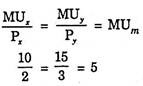
Thus 5 is the marginal utility of the last rupee spent on each of the two goods he purchases is the same, that is, Rs. 5.
Consumers’ equilibrium is graphically portrayed in Fig. 5.3. Since marginal utility curves of the goods slope downward, curves depicting Mux/Px and MUy/Py also slope downward.
Thus when the consumer is buying OH of X and OK of Y, then:
![]()
Therefore, the consumer is in equilibrium when he is buying 6 units of X and 4 units of Y. No other allocating of money expenditure will yield greater utility than when he is buying 6 units of X and 4 units of commodity Y. Suppose the consumer buys one unit less of good X and one unit more of good Y.
This will lead to the decrease in his total utility It will be observed from Fig. 5.3 (a) that the consumption of 5 units instead of 6 units of commodity X means a loss in satisfaction equal to the shaded area ABCH and consumption of 5 units of commodity Y instead of 4 units will mean gain in utility by the shaded area KEFL. It will be noticed that with this rearrangement of purchases of the two goods, the loss in utility ABCH exceeds gain in utility KEFL. Therefore, his total satisfaction will fall as a result of this rearrangement of purchases.

Thus when the consumer is making purchases by spending his given income in such a way that MUx/Px = MUy/Py, he will not like to make any further changes in the basket of goods and will therefore be in equilibrium situation by maximizing his utility.
The above equimarginal condition for the equilibrium of the consumer can be stated in the following ways:
(i) A consumer is in equilibrium when he equalises the ratios of marginal utilities of goods and their prices with each other. In other words, he is in equilibrium when
![]()
(ii) By rearranging the above equation we find that a consumer is in equilibrium when he equalises the ratio of marginal utilities of goods with the ratio of corresponding prices for each pair of goods consumed, that is, when
![]() and so forth.
and so forth.
(iii) Since Mux/Px or MUy/Py measure the marginal utility of a rupee’s worth of each good consumed at the given price, consumer can be said to be in equilibrium when the marginal utility of the last rupee spent on each good purchased is equal. Marginal utility of the last rupee spent on a good means the marginal utility of a rupee’s worth of the good. Thus, consumer is equilibrium when he spends his given income on various commodities in such a way that utility from the last rupee spent on each good is the same.
If the marginal utility of the last rupee spent on each good is denoted by MUm, then equilibrium condition of consumer’s equilibrium can also be stated as under:
![]()
Derivation of the Demand Curve and the Law of Demand:
We now turn to explain how the demand curve and the law of demand is derived in the cardinal utility analysis. The demand curve or the law of demand shows the relationship between price of a good and its quantity demanded. Marshall derived the demand curves for goods from their utility functions. It should be further noted that in his cardinal utility analysis of demand Marshall assumed the utility functions of different goods to be independent of each other.
In other words, Marshallian technique of deriving demand curves for the goods from their utility functions rests on the hypothesis of additive utility functions, that is, utility functions of each good consumed by a consumer does not depend on the quantity consumed of any other good. In case of independent utilities or additive utility functions, the relations of substitution and complementarity between goods are ruled out.
Further, in deriving a demand curve or law of demand Marshall assumes that marginal utility of money to remain constant. The law of demand or the demand curve can be derived in two ways first, with the aid of law of diminishing marginal utility, and secondly, with the help of the law of equimarginal utility. We shall explain below these two ways of deriving the demand curve and the law of demand.
Derivation of Demand Curve from Law of Diminishing Marginal Utility:
In order to derive the demand curve (and accordingly law of demand) we measure marginal utility of a good in terms of money (i.e., in terms of rupees) as Marshall did. Measuring marginal utility in terms of money or rupees implies how much value in terms of rupees an individual places on the successive units of the commodity consumed. In other words, how much money a consumer is prepared to pay for a unit of commodity will measure the marginal utility of that unit of the commodity in terms of money?
The law of marginal utility states that as the quantity of a good with a consumer increase marginal utility of the good to him falls. In other words, the marginal utility curve of a good is downward sloping. Now, a consumer will go on purchasing a good until the marginal utility of the good equals the market price.
In other words, the consumer will be in equilibrium in respect of the quantity of the good purchased where marginal utility of the good equals its price. His satisfaction will be maximum only when marginal utility equals price. Thus the “marginal utility equal’s price” is the condition of equilibrium.
When the price of the good falls, downward-sloping marginal utility curve implies that the consumer must buy more of the good so that its marginal utility falls and becomes equal to the new price. It therefore follows that the diminishing marginal utility curve of a good implies the downward-sloping demand curve, that is, as the price of the good falls, more of it will be bought.
The whole argument will be more clearly understood from Fig. 5.4. In panel (a) of Fig. 5.4 the curve MU represents the diminishing marginal utility of the good measured in terms of money. In panel (b) of Fig. 5.4 we measure price on the Y-axis. Suppose the price of the good is OP1. At this price the consumer will be in equilibrium when he purchases Oq1 quantity of the goods since at Oq1 the marginal utility of good X equal to MUX is equal to the given price OP1.

Now, if the price of the good falls to OP2, the equality between the marginal utility and the price will be disturbed. Marginal utility MUX from good X at the quantity Oq1 will be greater than the new price OP2. In order to equate the marginal utility with the lower price OP2, the consumer must buy more of the good. It is evident from Fig. 5.4 that when the consumer increases the quantity purchased to Oq2 the marginal utility of the good falls to MU2 and becomes equal to the new price OP2.
Hence, at price OP2, consumer demands Oq2 amount of the commodity. Further, if the price falls to OP3, this is equal to the marginal utility MU3 of the good at the larger quantity Oq3. Thus at price OP3, the consumer will demand Oq3 quantity of the good X. It is in this way the downward-sloping marginal utility curve is transformed into the downward-sloping demand curve when we measure marginal utility of a good in terms of money. It is worth noting that negative segment of the marginal utility curve MUX will not constitute a part of the demand curve. This is because no rational consumer will buy any further units of the commodity which reduces his total utility and make marginal utilities negative.
It is thus clear that when the price of the good falls, the consumer buys more of the good so as to equate its marginal utility to the lower price. It follows therefore that the quantity demanded of a good varies inversely with price; the quantity rises when the price falls and vice-versa, other things remaining the same.
This is the famous Marshallian Law of Demand. It is quite evident that the law of demand is directly derived from the law of diminishing marginal utility. The downward-sloping marginal utility curve is transformed into the downward-sloping demand curve. It follows therefore that the force working behind the law of demand or the demand curve is the force of diminishing marginal utility.
Derivation of Law of Demand: Multi-Commodity Model:
We now proceed to derive the law of demand and the nature of the demand curve from the principle of equimarginal utility in case when a consumer spends his money income on more than one commodity. Consider the case of a consumer who has a certain given income to spend on a number of goods. According to the law of equimarginal utility, the consumer is in equilibrium in regard to his purchases of various goods when marginal utilities of the goods are proportional to their prices.
Thus, the consumer is in equilibrium when he is buying the quantities of the two goods in such a way that satisfies the following proportionality rule:
![]()
Where, MUm stands for marginal utility of money expenditure. Thus, in the equilibrium position, according to the above principle of equimarginal utility, the ratios of the marginal utility and the price of each commodity a consumer buys will equal the marginal utility of the last rupee spent on each good. It follows therefore that a rational consumer will equalise MUx/Px of good X with MUy/Py of good Y and so on.
Given that other things such tastes and preferences of a consumer, his income, prices of other related commodities remain constant, we consider the demand for good X. Assume the price of good X is equal to Px. The consumer will allocate his given money income on various goods he purchases so that MUx /Px = MUy/Py = MUm and so forth.
Let us suppose that price of good X falls. With the fall in the price of good X, the price of good Y, consumer’s income and his tastes remaining unchanged, the equality of MUx, /Px = MUy/Py or with MUm in general would be disturbed. With lower price of good X than before, MUx /Px > MUy/Py or MUx, /Px > MUm. (It is of course assumed that marginal utility of money expenditure in general (MUm) does not change as a result of the change in the price of one good).
Then, in order to restore the equality, marginal utility of good X has to be reduced which can be done only if consumer buys more of good X. It is thus clear from the equimarginal principle that as the price of a good falls, its quantity demanded will rise, other things remaining the same. This proves the law of demand which states that there is inverse relationship between price of a good and its quantity demanded. The operation of this law of demand makes the demand curve downward sloping.
4. Limitations of the Law of Equimarginal Utility:
Like other laws of economics, law of equimarginal utility is also subject to various limitations. This law, like other laws of economics, brings out an important tendency among the people. This-is not necessary that all people exactly follow this law in the allocation of their money income and therefore all may not obtain maximum satisfaction.
This is due to the following reasons:
1. For applying this law of equimarginal utility in the real life, consumer must weigh in his mind the marginal utilities of different commodities. For this he has to calculate and compare the marginal utilities obtained from different commodities. But it has been pointed out that the ordinary consumers are not so rational and calculating. Consumers are generally governed by habits and customs. Because of their habits and customs they purchase particular amounts of different commodities, regardless of whether the particular allocation maximizes their satisfaction or not.
2. For applying this law in actual life and equate the marginal utility of rupee obtained from different commodities, the consumers must be able to measure the marginal utilities of different commodities in cardinal terms. However, this is easier said than done. It has been said that it is not possible for the consumer to measure the utility cardinally.
Being a state of feeling and also there being no objective units with which to measure utility, it is cardinally immeasurable. It is because the immeasurability of utility in cardinal terms that consumer’s behaviour has been explained with the help of ordinal utility by J.R. Hicks and R.G.D. Allen. Ordinal utility analysis involves the use of indifference curves.
3. Another limitation of the law of equimarginal utility is found in case of indivisibility of certain goods. Goods are often available in large indivisible units. Because the goods are indivisible, it is not possible to equate the marginal utility of money spent on them. For instance, in allocating money between the purchase of car and food-grains, marginal utilities cannot be equated.
Car costs about Rs. 20,000 and is indivisible, whereas food-grains are divisible and money spent on them can be easily varied. Therefore, the marginal utility of rupee obtained from car cannot be equalised with that obtained from food-grains. Thus, indivisibility of certain goods is a great obstacle in the way of equalisation of marginal utility of a rupee from different commodities.
5. Critical Evaluation of Marshall’s Cardinal Utility Analysis:
Utility analysis of demand which we have studied above has been criticised on various grounds.
The following shortcomings and drawbacks of cardinal utility analysis have been pointed out:
1. Cardinal Measurability of Utility is Unrealistic:
Cardinal utility analysis of demand is based on the assumption that utility can be measured in absolute, objective and quantitative terms. In other words, it is assumed in this analysis that utility is cardinally measurable. According to this, how much utility a consumer obtains from goods can be expressed or stated in cardinal numbers such as 1, 2, 3, 4 and so forth. But in actual practice utility cannot be measured in such quantitative or cardinal terms.
Since utility is a psychic feeling and a subjective thing, it cannot therefore be measured in quantitative terms. In real life, consumers are only able to compare the satisfactions derived from various goods or various combinations of the goods. In other words, in the real life consumer can state only whether a good or a combination of goods gives him more, or less, or equal satisfaction as compared to another. Thus, economists like J.R. Hicks are of the opinion that the assumption of cardinal measurability of utility is unrealistic and therefore it should be given up.
2. Hypothesis of Independent Utilities is Wrong:
Utility analysis also assumes that utilities derived from various goods are independent. This means that the utility which a consumer derives from a good is the function of the quantity of that good and of that good alone. In other words, the assumption of independent utilities implies that the utility which a consumer obtains from a good does not depend upon the quantity consumed of other goods; it depends upon the quantity purchased of that good alone. On this assumption, the total utility which a person gets from the whole collection of goods purchased by him is simply the total sum of the separate utilities of the good. In other words, utility function is additive.
Neoclassical economists such as Jevons, Menger, Walras and Marshall considered that utility functions were additive. But in the real life this is not so. In actual life the utility or satisfaction derived from a good depends upon the availability of some other goods which may be either substitute for or complementary with it. For example, the utility derived from a pen depends upon whether ink is available or not.
On the contrary, if you have only tea, then the utility derived from it would be greater, but if along with tea you also have the coffee then the utility of tea to you would be comparatively less. Whereas pen and ink are complements with each other, tea and coffee are substitutes for each other. It is thus clear that various goods are related to each other in the sense that some are complements with each other and some are substitutes for each other. As a result of this, the utilities derived from various goods are interdependent, that is, they depend upon each other.
Therefore, the utility obtained from a good is not the function of its quantity alone but also depends upon the availability or consumption of other related goods (complements or substitutes). It is thus evident that the assumption of the independence of utilities by Marshall and other supporters of cardinal utility analysis is a great defect and shortcoming of their analysis. The hypothesis of independent utilities along with the assumption of constant marginal utility of money reduces the validity of Marshallian demand theorem to the one-commodity model only.
3. Assumption of Constant Cardinal Utility of Money is not Valid:
An important assumption of cardinal utility analysis is that when a consumer spends varying amount on a good or various goods or when the price of a good changes, the marginal utility of money remains unchanged. But in actual practice this is not correct. As a consumer spends his money income on the goods, money income left with him declines. With the decline in money income of the consumer as a result of increase in his expenditure on goods, the marginal utility of money to him rises.
Further when the price of a commodity changes, the real income of the consumer also changes. With this change in real income, marginal utility of money will change and this would have an effect on the demand for the good in question, even though the total money income available with the consumer remains the same. But utility analysis ignores all this and does not take cognizance of the changes in real income and its effect on demand for goods following a change in the price of a good.
It is because of assuming constant marginal utility of money that Marshall ignored the income effect of the price change and this prevented Marshall from understanding the composite character of the price effect (that is, price effect being sum of substitution effect and income effect).
Moreover, as shall be seen later, the assumption of constant marginal utility of money together with the hypothesis of independent utilities renders the Marshall’s demand theorem to be valid in case of one commodity only. Further, it is because of the constant marginal utility of money and therefore the neglect of the income effect by Marshall that he could not explain Giffen Paradox.
According to Marshall, utility from a good can be measured in terms of money (that is, how much money a consumer is prepared to sacrifice for a good). But, to be able to measure utility in terms of money, marginal utility of money itself should remain constant. Therefore, assumption of constant marginal utility of money is very crucial in Marshallian demand analysis.
On the basis of constant marginal utility of money Marshall could assert that “utility is not only” measurable in principle but also “measurable in fact”. But, as we shall see below, in case consumer has to spread his money income on a number of goods, there is a necessity for revision of marginal utility of money with every change in the price of a good. In other words, in a multi-commodity model marginal utility of money does not remain invariant or constant.
Now, when it is realised that marginal utility of money does not remain constant, then Marshall’s belief that utility is measurable in fact in terms of money does not hold good. However, if in marginal utility analysis, utility is conceived only to be measurable in principle and not in fact, then it practically gives up cardinal measurement of utility and comes near the ordinal measurement of utility.
4. Marshallian Demand Theorem cannot Genuinely be Derived Except in a One Commodity Case:
J.R. Hicks and Tapas Majumdar have further criticised the Marshallian utility analysis on the ground that “Marshallian demand theorem cannot genuinely be derived from the marginal utility hypothesis except in a one-commodity model without contradicting the assumption of constant marginal utility of money.”
In other words, Marshall’s demand theorem and constant marginal utility of money are incompatible except in a one commodity case. As a result, Marshall’s demand theorem cannot be validly derived in the case when a consumer spends his money on more than one good.
Thus, we see that marginal utility of money cannot be assumed to remain constant when the consumer has to spread his money income on a number of goods. In case of more than one good, Marshallian demand theorem cannot be genuinely derived while keeping the marginal utility of money constant.
If, in Marshallian demand analysis, this difficulty is avoided “by giving up the assumption of constant marginal utility of money, then money can no longer provide the measuring rod, and we can no longer express the marginal utility of a commodity in units of money. If we cannot express marginal utility in terms of common numeraire (which money is defined to be), the cardinality of utility would be devoid of any operational significance.”
5. Cardinal Utility Analysis does not Split Up the Price Effect into Substitution and Income Effects:
The third shortcoming of the cardinal utility analysis is that it does not distinguish between the income effect and the substitution effect of the price change. We know that when the price of a good falls, the consumer becomes better off than before, that is, a fall in price of a good brings about an increase in the real income of the consumer.
In other words, if with the fall in price the consumer purchases the same quantity of the good as before, then he would be left with some income. With this income he would be in a position to purchase more of these good as well as other goods. This is the income effect of the fall in price on the quantity demanded of a good.
Besides, when the price of a good falls, it becomes relatively cheaper than other goods and as a result the consumer is induced to substitute that good for others. This results in the increase in the quantity demanded of that good. This is the substitution effect of the price change on the quantity demanded of the good.
With the fall in price of a normal good, the quantity demanded of it rises because of income effect and substitution effect. But marginal utility analysis does not make clear the distinction between the income and the substitution effects of the price change. In fact, Marshall and other exponents of cardinal utility analysis ignored income effect of the price change by assuming the constancy of marginal utility of money.
Thus, marginal utility analysis does not tell us about how much quantity demanded increases due to income effect and how much due to substitution effect as a result of the fall in price of a good. J.R. Hicks rightly remarks, “That distinction between income effect and substitution effect of a price change is accordingly left by the cardinal theory as an empty box which is crying out to be filled.”
6. Marshall Could not Explain Giffen Paradox:
By not visualising the price effect as a combination of substitution and income effects and ignoring the income effect of the price change, Marshall could not explain Giffen Paradox. He treated it merely as an exception to his law of demand. In constant to it, indifference curves analysis has been able to explain satisfactorily the Giffen good case.
According to indifference curves analysis, in case of Giffen Paradox or Giffen good negative income effect of the price change is more powerful than the substitution effect so that when the price of a Giffen good falls the negative income effect outweighs the substitution effect with the result that quantity demanded of it falls.
Thus, in case of a Giffen good quantity demanded varies directly with the price and the Marshall’s law of demand does not hold good. It is because of the constant marginal utility of money and therefore the neglect of the income effect of price change that Marshall could not explain why the quantity demanded of a Giffen good falls when its price falls, and rises when its price rises. This is a serious lacuna in Marshallian’s utility analysis of demand.
7. Cardinal Utility Analysis Assumes too Much and Explains too Little:
Cardinal utility analysis is also criticised on the ground that it takes more assumptions and also more restrictive ones than those of ordinal utility analysis of indifference curves technique. Cardinal utility analysis assumes, among others, that utility is cardinally measurable and also that marginal utility of money remains constant.
Hicks-Allen’s indifference curve analysis does not take these assumptions and even then it is not only able to deduce all the theorems which cardinal utility analysis can but also deduces a more general theorem of demand. In other words, indifference curve analysis explains not only that much as cardinal utility analysis but even goes further and that too with fewer and less restrictive assumptions.
Taking less restrictive assumption of ordinal measurement of utility and without assuming constant marginal utility of money, indifference curve analysis is able to arrive at the condition of consumer’s equilibrium, namely, equality of marginal rate of substitution (MRS) with the price ratio between the goods, which is similar to the proportionality rule of Marshall. Further, since indifference curve analysis does not assume constant marginal utility of money, it is able to derive a valid demand theorem in a more than one commodity case.
Indifference curve analysis is able to explain Giffen Paradox which Marshall with his cardinal utility analysis could not. In other words, indifference curve analysis clearly explains why in case of Giffen goods, quantity demanded increases with the rise in price and decreases with the fall in price. Indifference curve analysis explains even the case of ordinary inferior goods (other than Giffen goods) in a more analytical manner.
It may be noted that even if the valid demand theorem could be derived from the Marshallian hypothesis, it would still be rejected because “better hypothesis” of indifference preference analysis was available which can enunciate a more general demand theorem (covering the case of Giffen goods) with fewer, less restrictive and more realistic assumptions.
Because of the above drawbacks, utility analysis has been given up in modern economic theory and demand is analysed with indifference curves.