Consumer Behavior Analysis: Ordinal Utility Approach

Modem economists, particularly Hicks gave ordinal utility concept to analyze consumer behavior.

He has used a tool, called indifference curve, for consumer behavior analysis.

The ordinal utility approach is based on the following assumptions:

i. Rationality:

Implies that a consumer is a rational being and aims at maximizing the total satisfaction given the income and prices of goods and services.

ii. Ordinal Utility:

Assumes that utility is expressible only in ordinal terms. This implies that a consumer is only able to express his/her preference for goods.

iii. Transitivity and Consistency of Choice:

Implies that consumer choices are assumed to be transitive and consistent. The transitivity of choice means that if a consumer prefers A to B and B to C, he/she would prefer A to C. On the other hand, the consistency of choice means that if a consumer prefers A to B in one period, he or she cannot prefer B to A in another period.

iv. Non-satiety:

Implies that a consumer is assumed to be non-satisfied. In other words, it is assumed that consumer does not reach the level of satisfaction by consuming a good and always prefers a large quantity of goods.

v. Diminishing Marginal Rate of Substitution:

Acts as an important concept in indifference curve analysis. Marginal rate of substitution implies the rate at which a consumer is willing to substitute one good (X) for another good (Y), so that the total satisfaction remains the same.

Meaning of Indifference Curve:

Indifference curve is defined as the locus of points on the graph each representing a different combination of two substitute goods, which yield the same utility or level of satisfaction to a consumer. The combinations of goods give equal satisfaction to a consumer.

Therefore, a consumer is indifferent between any two combinations of two goods when it comes to making a choice between them. When these combinations are plotted on the graph, the resulting curve is called indifference curve. This curve is also called as iso-utility curve or equal utility curve.

Let us learn the indifference curve through a schedule.

Table-3 shows the indifference schedule for goods X and Y:

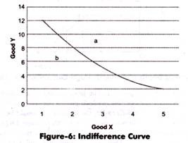
Table-3 depicts that a consumer starts with one unit of good X and 12 units of good Y. For gaining an additional unit of X, he/she sacrifices 4 units of good Y, so that the level of satisfaction remains the same. Similarly, we get the combinations of 3X+ 5Y, 4X+ 3Y, 5X+2Y. The consumer’s satisfaction remain same whichever the combination of goods. This schedule of combinations can be show n graphically on indifference curve. The quantity of good X is measured on X-axis and quantity of good Y is shown on Y- axis.

Figure-6 shows indifference curve:

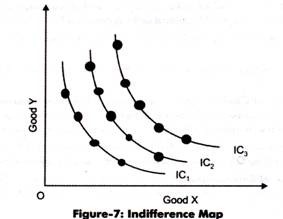
In Figure-6, point b shown below and left of the indifference curve would give less satisfaction and point a above the indifference curve would be more preferred than combinations. A description of consumer’s preferences is represented on indifference map that consists of a set of indifference curves. Indifference map shows the indifference curves ranked in order of preferences of consumers.

Figure-7 shows the indifference map:

All the combinations on indifference curve IC₁, IC₂, and IC₃ give equal level of satisfaction where IC₃ is more preferred than IC₂ and IC₂ is more preferred than IC₁. A higher indifference curve represents a higher level of satisfaction.

However, the indifference curve does not indicate the exact value of level of satisfaction. This is because indifference curve is based on the concept of ordinal utility, which states that only the qualitative differences in levels of satisfaction can be stated by the consumer.

Marginal Rate of Substitution:

An indifference curve is formed when one good is substituted for other. Marginal Rate of Substitution (MRS) refers to a rate at which one good is substituted for other, while keeping the level of satisfaction of a consumer constant. In other words, MRS between two goods X and Y is defined as the quantity of X which is required to replace Y or quantity of Y required to replace X, so that the total utility remains same.

It is expressed as:

MRS x,y = ∆Y/∆X

MRS is called the slope of indifference curve.

Let us discuss the concept of MRS through a schedule and graph.

Table-4 shows the schedule of MRS between goods X and Y:

In Table-4, it can be seen the MRS is diminishing. This is because the basic assumption of the ordinal utility concept is that MRS diminishes.’ This implies that a consumer sacrifices some unit of a good X or Y when substituting X for Y or Y for X.

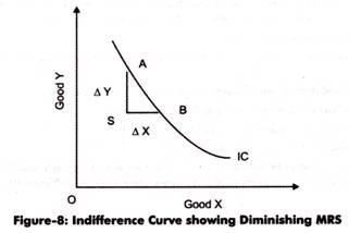
The diminishing MRS x,y attained from the combination of good X and Y is shown in Figure-8:

From Figure-8, it can be seen that the consumer is ready to sacrifice AS of Y to gain SB of X. Thus, MRS = AS/SB= ∆ Y/∆ X. It can be noted from schedule (Table-4) and graph (Figure-8) that MRS falls as more and more of good X is consumed. The reason for convex shape of indifference curve is diminishing MRS.

The MRS diminishes because of the two main reasons. Firstly, in indifference curve, the combination of two goods is such that quantity of one good is more than the quantity of another good. Thus, consumer is ready to sacrifice more of good whose quantity is large. When the consumer’s stock of good Y is large than good X, he/she would be willing to give up large amount of good Y to gain more of X and vice versa; therefore, MRS falls.

MRS diminishes because two goods X and Y are not perfect substitutes of each other. If they are perfect substitutes, then indifference curve would be a straight line showing constant MRS. The increase in quantity of one and decrease in quantity of other would not make any difference in the marginal significance of goods. However, in case of imperfect substitutes, the consumer is required to sacrifice additional units of Y to gain increasing units of X to maintain the level of satisfaction. Thus, MRS decreases.

Properties of Indifference Curve:

As discussed earlier, indifference curve plays an important role in analyzing consumer behavior through ordinal utility concept.

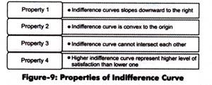
It has four main properties, which are shown in Figure-9:

The properties of indifference curves (as shown in Figure-9) are explained as follows:

i. Indifference curves slopes downward to the right:

Implies that indifference curves have a negative slope. This property is based on the assumption of non-satiation, which refers that a consumer is never satisfied and prefers more of goods to less of it.

Indifference curve being downward sloping implies two things, which are as follows:

a. Two goods can be substituted for each other

b. As quantity of one good increases, the quantity of another good decreases, so that the consumer stays at the same level of satisfaction

This property can be explained through two different situations, which are as follows:

a. If indifference curve is horizontal straight line (parallel to the X-axis)

b. If indifference curve is vertical straight line (parallel to the Y-axis)

c. If indifference curve is upward sloping to the right

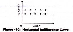
If indifference curve is horizontal straight line parallel to X-axis, it implies that good Y would remain constant and there would be change in the quantity of good X.

The horizontal indifference curve is shown in Figure-10:

In Figure-10, it can be seen that OP is the fixed amount of good Y and amount of good X is successively larger. It is clear that the consumer always prefers a large quantity of goods. Indifference curve states that at different combinations, consumer is indifferent and his/her total utility remains the same.

However, in this case, a consumer would prefer combination E as it is offering more quantity of X with fixed quantity of Y. The combinations A, B, C, D, and E do not yield same satisfaction to the consumer. Thus, it can be said that the indifference curve cannot be a horizontal straight line.

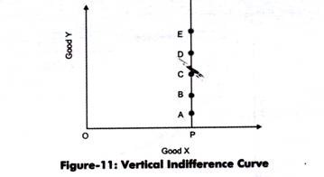
Similarly, indifference curve cannot be a vertical straight line parallel to Y axis. It would mean that amount of good Y in the combination increases and amount of good X remains the same. As shown in Figure-10, the combinations A, B, C, D, and E do not yield same satisfaction to the consumer, thus, it is proved that indifference curve cannot be a vertical straight line.

Figure-11 shows the vertical indifference curve:

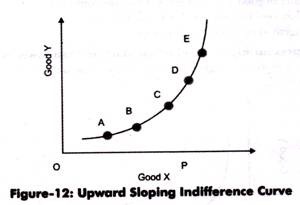
If the indifference curve is upward sloping to the right, it will imply that amount of both the goods offering larger quantities would be preferred. According to indifference curve, the combinations give equal satisfaction; further means that the combination offering large quantities would be equal to combination offering smaller quantities. This would that consumer is irrational. Thus, it is proved that indifference curve cannot slope upward to the right.

Figure-12 shows the upward sloping indifference curve:

Thus, indifference curve must slope downward to show that when the quantity of one good in a combination increases, the quantity of other good must fall, so that the level of satisfaction remains unchanged.

ii. Indifference curve is convex to the origin:

Implies that MRS decreases and two goods are imperfect substitutes of each other. A convex indifference curve implies that MRS of good X for the good Y falls as more quantity of X is substituted for good Y.

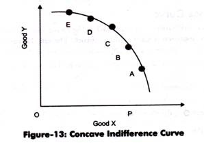
If indifference curve is concave to the origin, it would mean that MRSxy increases as more and more of goods X and Y are consumed. This leads to failure of assumption that MRSxy diminishes. Thus, indifference curve must be convex to the origin.

Figure-13 shows the concave indifference curve:

iii. Indifference curve cannot intersect each other:

Implies that only one indifference curve can pass through a point in indifference map.

If two indifference curves intersect each other, two impossible conclusions are achieved, which are as follows:

a. Two equal combinations of goods yield different levels of satisfaction

b. Two different combinations of goods yield same satisfaction

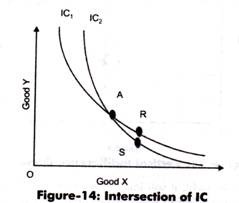
If two indifference curves intersect each other, the assumption of transitivity is contradicted. Let us learn this diagrammatically.

Figure-14 shows the intersection of two indifference curves:

As shown in Figure-14 two indifference curves IC₁ and IC₂ intersect at point C. As all the combinations at indifference curve give equal satisfaction. Therefore, it can be implied from Figure-14 that A=R and A=S. This means that R=S, which is wrong It can be seen that point R gives more of good Y than point S. Thus, the consumer would prefer R to S in terms of satisfaction therefore, it can be concluded that two indifference curves cannot intersect each other. The same reason applies if two indifference curves touch or are tangent to each other at any point.

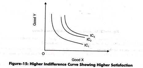
iv. Higher indifference curve represent higher level of satisfaction than lower one:

Implies that the combinations that lie on higher indifference curve represents higher satisfaction level than the combinations on lower indifference curves.

This can be explained through Figure-15:

In Figure-15, it can be seen that all combinations on IC₂ give more satisfaction than combinations on IC₁. This is because every combination on IC₂ provides more of both the goods than combination on IC₁.

Criticism of Indifference Curve:

Prof. D.H. Robertson was of the view indifference curve approach is like an old wine in a new bottle and tells nothing new. He further advocates that indifference curve approach is same as utility theory. The only change which Hick has made is in use of words, MRS instead of marginal utility.

The indifference curve approach is criticized on the following grounds:

a. Assumes that there are only two goods in indifference curve approach. This is not true in the real world as a consumer consumes variety of goods.

b. Fails to provide a clear explanation of consumer behavior

c. Provides combinations that are not based on the principles of economics

d. Ignores risk and uncertainty while analyzing the consumer behavior

Concept of Budget Line:

A consumer prefers to reach the highest possible indifference curve on indifference map to attain satisfaction. However, he/she suffers from two constraints, namely, limited income and price of goods. The lack of income is called budgetary constraint.

The budget equation is expressed as:

Px.Qx + Py.Qy = M

Px and Py are the prices of goods X and Y

Qx and Qy are the quantities of goods X and Y

M= money income of the consumer

The budget equation states that the total expenditure cannot exceed the total income.

The quantities can be derived as:

Qx = M/Px-Py/Px. Qy

Qy = M/Py-Px/Py.Qx

When these quantities are plotted on a graph, a budget line is obtained, which is also called price line. The indifference curve shows preferences of combination of two goods where the actual choice of preferences depends on income.

Budget line is the combination of two goods that can be purchased with a given money income and prices of goods. The consumer behavior is well depicted by the budget line. The budget line is drawn as a continuous line that identifies alternatives from which a consumer selects an appropriate combination of goods.

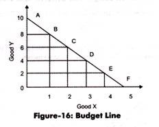
Suppose the income of a consumer is Rs. 60. He/she wants to consume goods X and Y. The price of good X is Rs. 12 and the price of good Y is Rs. 6.

The various preferences of X and Y that can be purchased from the given income and prices are shown in Table-5:

From Table-5, it can be seen in combination A the whole amount of Rs. 60 is spent on purchase of quantity Y. In such a ca.se, the consumer buys 10 units of good Y and nothing is Left for purchasing good X. Similarly, combination F shows that if the consumer spends the entire amount on good X, then he/she is able to purchase 5 units of good X and nothing of good Y. The combinations B to E show the combined quantities of good X and good Y. For instance, in combination B, the consumer would purchase 8 units of good Y and 1 unit of good X.

With the help of preferences, the budget line is drawn, which is shown in Figure-16:

In Figure-16, budget line AF shows various combinations of good X and Y that a consumer can purchase from his or her given budget. The combinations are shown by points A, B, C, D, E, and F that can be purchased with the given budget. If a consumer buys the combination of goods inside the budget line AF, then the total expenditure comes out to be less than the given budget.

Slope of Budget Line:

The slope of a budget line shows how many units of Y are sacrificed to get more units of X.

It can be expressed as:

Slope of the Budget Line = ∆Y/∆X

For instance, from Figure-16, it can be seen that the slope at point B equals to 1 unit of X for 2 units of Y. It implies that 2 units of good X. It should be noted that the slope of budget line is negative. For instance, slope is -2 in case of preference B.

The slope of the budget line (Figure-16) would be given as:

∆Qy/∆Qx = OA/OF

When X = 0, OA = M/Py

When Y = 0, OF = M/Px

Thus, OA/OF = Px/Py

Therefore, it can be said that the slope of the budget line equals to the price ratio of two goods.

Shifts in Budget Line:

The budget line is determined by the income level of consumers and prices of goods in the market. The budget line shifts if there is a change in the income and prices. Let us take the both cases one by one.

Case 1: Change in Income:

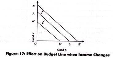
Suppose there is a charge in the income of the consumer and the price of the goods remain same. The budget line would shift from the original position. If there is a rise in income, the budget line would shift upward to the right. On the other hand if there is a fell in income, the budget line would shift downward to the left.

Figure-17 shows a shift in budget line due to change in income:

From Figure-17, it can be seen that a rise in income shifts the budget line from AB to A’B’ and a fall in income shifts the budget line from AB to A”B”.

Case 2: Change in Prices:

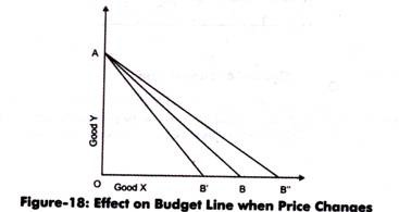
Suppose there is a change in the price of a good, say good X, and the income and price of good Y are constant. If there is a fall in the price of good X, then the consumer can buy more of good X with the same income.

Figure-18 shows the shift in the budget line due to change in the price of good X:

As shown in Figure-18, when the price of good X falls, this would make the budget line too move flatter and rightward from “AB to AB”. In case, the price of good X increases, the budget line shifts to the left that is from AB to AB’.

Consumer’s Equilibrium through Indifference Curve and Budget Line:

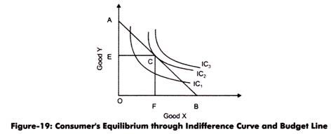
Consumer’s equilibrium is the point at which consumer attains maximum satisfaction. A consumer is said to be in equilibrium when the budget line touches indifference curve, with given price and income.

The consumer’s equilibrium through indifference curve and budget line is shown in Figure-19:

In Figure-19, there are three indifference curves IC1, IC2 and IC3. The budget line AB is tangent to IC2 at point C. At this level, a consumer attains maximum satisfaction level at OE units of good Y and OF units of good X. This is the first condition for the consumer to be in equilibrium that indifference curve should touch the budget line. The second condition is that the slope of budget line should be equal to the slope of indifference curve.

Slope of budget line =Px/Py

Slope of indifference curve= ∆Y/∆X = MRSxy

Thus, Px/Py = MRSxy