Classical Model of Employment: An Overview

Let us make an in-depth study of the features, generalised form, summary and criticism of classical model of employment.

Features of Classical Model:

(i) Effect of a Change in Money Supply:

An important feature of the classical model is that employment, real wage rate, real income and the interest rate are independent of the quantity of money.

If the quantity of money is changed by the monetary authority, disequilibrium will be created in the money market only. In terms of the system of equations we can write that equation (1) – (3) will remain unchanged when money supply changes.

Thus, the level of income, the level of employment and the real wage rate will not be affected when money supply changes. The equilibrium rate of interest as determined by equations (4) – (6) will also remain unchanged. Equation (7) – (9) will only be affected when money supply changes. Equations (7) – (9) can be written as a single equation M₀ = kPY, where k and Y remain constant.

Hence, to maintain equilibrium in the classical system P must increase when money supply (M₀) increases. P will increase in the same proportion in which money supply increases. Since the real wage rate remains unaffected, it means money wage rate must increase in the same proportion in which the price level increases.

Thus, when the supply of money changes the real variables in the system will remain unchanged while monetary variables will change proportionately. In this sense, money is said to be neutral in the classical model.

Suppose the money supply is doubled from M₀ to 2M₀. Then, in Fig 7.3, the rectangular hyperbola of part III will shift to the right to 2M₀/k = PY. The equilibrium remains unchanged at Y_f but the equilibrium price level is doubled to 2P_f. Since the real wage rate in part I remains unaffected, the real wage line in part IV remains at the same level. From this line we get the money wage rate given the price level which is now 2P_f and the money wage rate becomes 2W_f.

Thus, an increase in the quantity of money affected only parts III and IV of the Fig. 7.3. But it has no impact on parts I, II and V in Fig. 7.3. Similarly, if money supply decreases, price and money wages will be reduced in the same proportion. Thus, in the classical model money is a “veil” which leaves real variable of the system unaffected when money supply is changed.

(ii) Effect of a Shift of the Production Function:

We can see the effect of an upward shift of the production function in the classical model. The upward shift implies an increase in the marginal product of labour. As the marginal product of labour increases, the labour demand curve shifts to the right as in part I in Fig. 7.3. In part II of Fig. 7.3, the production function shifts from Y to Y₂, we get a new marginal product curve MPL₂ in part I.

The equilibrium real wage rate increases from (W/P)_f to (W/P)₂ and the equilibrium employment increases from N_f to N₂. Output increases from Y_f to Y₂ both because of higher productivity and larger employment. When money supply remains unchanged, the price level falls from P_f to P₂ in part III.

Since the real wage rises the real wage line rotates from (W/P)_f to (W/P)₂ . As can be seen from the Fig. 7.3, when the price level falls money wage rate also falls from W_f to W₂. However, depending on the slopes of the various functions, the new money wage might also be higher than the old. The real wage rate will definitely be higher as well.

(iii) Shift of Labour Supply Curve:

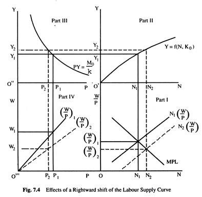
We can see the effects of a rightward shift of the labour supply curve in the classical model. We assume that the money supply remains unchanged when labour supply curve shifts upward. The effects can be analysed with the help of the Fig. 7.4.

In part I of Fig. 7.4, the labour supply curve has shifted from N₁ (W/P) to N₂ (W/P) .This has the effect of increasing the equilibrium level of employment from N₁ to N₂ and reducing the equilibrium real wage rate from (W/P)₁ to (W/P)₂. In part II, we can see that when the level of employment has increased from N₁ to N₂, the level of output has also increased from Y₁ to Y₂.

In part III, we can see that as the level of output increases from Y₁ to Y₂ the equilibrium price level decreases from P₁ to P₂. As the real wage rate has decreased from (W/P)₁ to (W/P)₂ j the real wage line (W/P)₂ has lower slope than the real wage line (W/P)₁. From the real wage line (W/P)₂ it can be seen that the money wage rate is lower at W₂, when the price level has come down to P₂.

Thus, the effect of an increase in the supply of labour can be summarised as below: a lower real wage, a larger employment, a larger output, a lower money wage rate and the lower price level. The rate of interest will remain unaffected. It is interesting to note that a change in the real variable affects the money variable as well.

A Generalised Classical Model of Income and Employment:

Let us now consider a classical model which is different from simple classical model in many respects. In the simple model we assumed that the determination of interest rate is independent of the determination of the level of income. The interest rate is determined by saving and investment which are functions of the rate of interest.

Now, suppose that saving and investment depend not only on the rate of interest but also on the level of income. We have the following general saving and investment functions: S = S(r, Y) such that δS/δr > 0. δS/δY > 0. I = l(r, Y) where δI/δr < 0 and δI/δY > 0. And S = I is the equilibrium condition. In this general model the determination of the interest rate is not independent of the level of income since the level of income enters in the model as a variable in the saving and investment functions.

Again, in the simple classical model, it is assumed that the demand for money is a function of income only. It is independent of the rate of interest. Now, we take into consideration the speculative demand for holding money which is also a function of the rate of interest. Thus, we modify our analysis by assuming that the demand for money is a function not only of the level of income but also a function of interest rate. We now introduce the speculative demand for money into the classical model.

The money demand function may be written as follows:

M_d/P = L(r, Y), where M_d/P is the demand for real money balances. This is the same as the liquidity preference function of Keynes which states that the demand for money is a function of both the level of income and the rate of interest. This means that the demand for real money balances is inversely related with the rate of interest and directly related to the level of income which means that δ(M_d/P)/δY > 0 and δ(M_d/P)/δr < 0.

We now assume that the money wages and prices are perfectly flexible and the perfect competition prevails in the economy. Entrepreneurs try to maximise their profit. Total capital stock is constant. The volume of output depends on the level of employment, given the capital stock. The aggregate production function can be written as: Y = f(N, K₀) where N is employment, K₀ is a given stock of capital. We also assume that the demand for labour is the value marginal product of labour and the supply of labour is a positive function of real wage rate.

The generalised classical model can be written as:

1) Y = f(N, K₀)

2) dY/dN = W/P

3) N = N (W/P)

4) M_d/P = L(r, Y)

5) M_s = M₀

6) M_d = M_s

7) S = S(r, Y)

8) I = I(r, Y)

9) S = I

In this model, there are 9 equations and 9 unknowns: Y, N, W, P, M_d, M_s, S, I, r. Hence the system is deterministic. Now, let us consider the nature of the system. Equations (1) – (3) determine the values of Y, N and W/P, three unknowns. This is a full employment equilibrium because of the as­sumption of perfect flexibility of money wages and prices.

Thus, full em­ployment level of income is automatically achieved. In the last three equations (7) – (9), we consider first the saving functions S = S(r, Y) which has three unknowns, we can get relationship between S and r assuming that Y is constant at a certain level. Simi­larly, we can get one investment function relating investment and interest rates for one level of income.

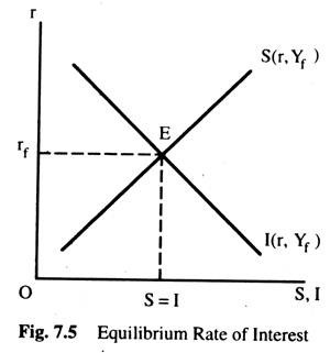
Thus, we get the saving and invest­ment functions corresponding to the level of income Y_f. At this point of intersection between the saving and investment functions the equilibrium rate of interest is determined. This is illustrated in Fig. 7.5.

In Fig. 7.5, the investment function is l(r, Y_f) which corresponds to the full em­ployment level of income, Y_f and the saving function is S(r, Y_f) which also corresponds to the full employment level of income Y_f. They intersect at the point E which gives us the equilibrium level of the rate of interest r_f. At this rate of interest, saving equals investment at full employment level of income and employment.

Let us now consider the money market equations (4) to (6). These equations can be written as M₀/P = L(r, Y). or M₀ = PL(r, Y)……………. (10).

It is a single equation with only one unknown, since rand Fare already known. It is possible to determine the equilibrium P level from the demand for money function even if it is a function of interest rate.

The price level is determined from the equilibrium condition of the money market so long as money wages and prices are assumed to be perfectly flexible. In other words, when the money wages and prices are flexible, liquidity preference function determines the price level.

This is still a classical model since its conclusions are the same as those of the simple classical model. Like the simple classical model, full employment equilibrium is automatically achieved in the labour market. Underemployment equilibrium is not possible in this system.

Moreover, like the classical model, the rate of interest is also determined by the saving and investment functions and the price level is determined from the equilibrium of the money market where money demand function is dependent on the rate of interest.

Consider the effects of a change in money supply in this model. Equations (1) to (3) will remain unaffected when money supply increases which means equilibrium levels of employment and income will remain unchanged when money supply increases.

As a result, the saving and investment functions and, hence, the equilibrium rate of interest will remain unaffected. Only the equilibrium condition of the money market will be affected as the supply of money increases. The equilibrium condition of the money market can be written as M₀ = PL(r, Y).

In this equation r and Y will remain unaffected and thus the only variable that will be affected when the money supply changes is the price level. The price level will increase in the same proportion as increase in money supply. This result is not different from the simple classical model. Thus, money is also neutral in this model.

It is clear from this analysis that even if we introduce a few modifications in the simple classical model the properties of the classical model remain unchanged as long as equations (1) – (3) are retained i.e. we assume perfectly flexibility of wages and prices. These equations (1) – (3) may be called the heart of the classical model. So long as they remain intact the classical conclusion will not change.

However, in this modified version, there are two exceptions where full employment will not be achieved even if money wages and prices are perfectly flexible.

Two Exceptional Cases:

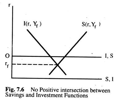
First, we consider the situation where the saving and investment functions are such that there is no positive intersection between them as in Fig. 7.6 to achieve full employment.

The saving function at full employment intersects the investment function at full employment to produce a negative rate of interest r_f. That is, a negative at full employment. Since the rate of interest cannot be negative, the full employment cannot be achieved under this circumstances. Here, at all positive rate of interest, saving is greater than invest­ment at full employment.

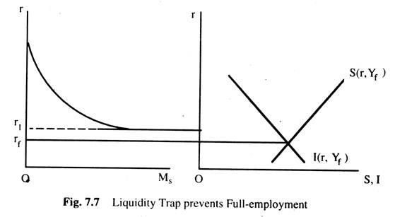
The shapes of saving and invest­ment functions are such that they prevent full employment being achieved in this situation. In other words, the interest- inelasticity of investment and saving functions cannot give full employment in this case. The second situation is where the speculative demand function for money may act as an obstacle to achieve full employment. We know that there is a lower limit below which interest rate may not fall.

This lower limit is set by the liquidity trap where the speculative demand for money becomes horizontal. Now, if the rate of interest required to achieve full employment is less than the rate of interest permitted by the liquidity trap situation, then full employment may not be achieved, as the Fig. 7.7 shows.

The rate of interest required to achieve full employment is r_f. But the minimum rate of interest permitted by the liquidity trap situation is r₁. To achieve full employment, we require the rate of interest r_f, but the liquidity trap situation does not allow the rate of interest to fall below r₁.

In this case, the speculative demand for money function prevents the economy to achieve full employment. Apart from these two special cases, full employment will be automatically achieved in this modified classical model as in simple classical model. Hence, this model may also be described as a classical model.

Summary of the Classical Theory of Full-employment:

1) A basic result of the classical economics was that, given flexible wages and prices, a competitive market economy would operate at full employment, which means that economic forces would always be generated to ensure that the demand for their labour would always equal its supply.

2) The equilibrium levels of income and employment were believed to be determined mainly in the labour market. The demand curve for labour (=MPL in a competitive economy) shows the relationship between real wage and the employer’s demand for labour. This relationship is inverse: the lower the real wage, the more workers will be employed. The supply curve for labour shows a direct relationship between the real wage and supply of labour by households; the higher the real wage, the greater the supply of labour.

3) Suppose that the wage rate is flexible and that the economy is sufficiently competitive to ensure that labour market equilibrium. Can we be sure that aggregate demand will be sufficient to take up the full-employment output produced? The classical economists answer is yes—whatever the full employment level of output, the income generated in producing it will necessarily lead to spending which will be just sufficient to purchase the entire output produced. The supply will create its own demand and there can be no overproduction.

This is the famous Say’s law which shows that households receive income equal to the value of goods and services produced. Part of this income they spend and part they save Consumption demand falls short of the total value of production by the amount of savings. This shortfall is made up by the investment demand and so long as investment and saving are equal, aggregate demand will equal the total value of goods and services produced.

The classical economists argued that, given a flexible rate of interest and competitive market for loanable funds, savings and investment would always be made equal by changes in interest rates. For example, if savings exceeded investment, interest rates would fall, causing investment to rise and savings to be reduced.

Similarly, if investment exceeded savings, the demand for loanable funds would exceed their supply and this would push interest rate upwards, bringing forth more saving and reducing investment until they are equal again.

Thus, we can say that the classical system depends upon: (a) the de­pendence of investment and savings on the rate of interest, (b) the flexibility of wages, prices and interest rates, (c) the existence of competitive forces in the economy. Given these conditions, there could be no overproduction and full employment would be assumed.

Critisicm:

Keynes criticised the classical theory on the following grounds:

a) Savings depend mainly on the level of national income and are not much affected by changes in interest rates. Investment may be influenced by interest rates, but also depends on business expectations. Given this, it is unlikely that the rate of interest would ensure equality between planned savings and planned investment and thus Say’s law will no longer hold.

b) He argued that, because of monopoly power in both the goods and labour markets, wages and prices will tend to be inflexible, at least in the downward direction. This means that in a situation where saving exceeds investment so that aggregate demand is less than the total value of production, firms will reduce output and lay off workers. It is in this way that demand deficient unemployment is created.

c) He also argued that even if wages and prices are flexible, aggregate demand may not be sufficient to ensure full employment.

In the Keynesian theory, the level of real national income and employment is determined largely by the level of aggregate demand. This is really very different from the classical model where supply creates its own demand and in the Keynesian model, as we will analyse below, it is demand which determines how much is supplied.

The argument is that if firms find that they are producing more than, is being demanded, they will observe an involuntary increase in inventories of unsold goods and so will rectify this by cutting production and laying off workers.

National income will fall until the value of production is equal to the value of aggregate demand. If, however, firms find that they are producing less than what is demanded, they will experience an unwanted fall in inventories and so this time will try to increase output and hire more workers.

There will be one level of national income at which aggregate demand is equal to the total value of production, which is called the equilibrium level of income. An important point to remember is that, in the Keynesian model, the equilibrium level of income is not necessarily the same as the full employment level of income.

This is the reason Keynes called his theory a general theory — he regarded the classical theory as no more than the ‘special case’ whose equilibrium and full employment level of income coincided.