Classical Theory of Employment and Output (With Diagram)

To build up a classical macroeconomic model, here we will consider a particular framework within which the classical system can be studied.

This framework is composed of an aggregate production function, the labour market, the money market, and the goods market.

1. Employment-Output Determination: Labour Market:

Let us first consider the labour market where we deal with production function in which capital stock is fixed and labour is the variable input.

The aggregate production function is: Y = f (K , L) … (3.2)

where K denotes a constant capital stock and L denotes quantities of variable input, labour.

In the classical model, equilibrium level of output is determined by the employment of labour. The level of output and, hence, the level of employment is established in the labour market by the demand for and supply of labour.

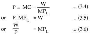
Assuming a profit-maximising economy, labour will be demanded up to the point where the revenue earned from selling the total product produced by the marginal unit of labour is equal to the MC of labour. MC of labour is equal to the money wage divided by the marginal product of labour, MP_L, i.e.,

MC = W/MP_L

The condition for profit maximisation is

where W is the money wage, P is the absolute price level, and W/P is the real wage.

We know that the MP curve for labour indicates the firm’s demand for labour. More labour is demanded at a lower wage. Thus, demand for labour depends inversely on real wage. The aggregate demand curve for labour is the horizontal summation of all individual firm’s demand curve for labour. Aggregate labour demand function, shown in equation (3.7), is also inversely related to the real wage rate. That is,

D_L=f (W-p) …(3.7)

Like labour demand, aggregate labour supply function also depends on the real wage rate, but in a direct manner. Thus,

S_L=g (W/P)… (3.8)

These relationships (equations 3.2, 3.7 and 3.8), together with the equilibrium condition for the labour market

D_L = S_{L …} (3.9)

determine output, employment and real wage in the classical system.

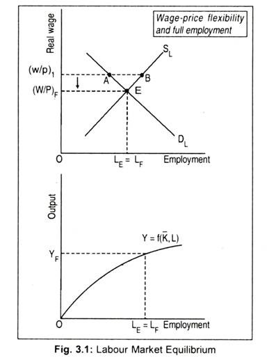
Equilibrium real wage rate and the equi­librium level of employment are determined at that point where the negative sloping la­bour demand curve cuts the positive sloping labour supply curve. Once we know the equi­librium level of employment from the aggre­gate production function we can derive the equilibrium level of output.

This is shown in Fig. 3.1. In the lower panel, aggregate produc­tion function has been shown. The intersec­tion between D_L and S_L curves at point E in the upper part of the figure determines the equilibrium level of employment (L_F) at the equilibrium real wage rate (W/P)_F. The equilibrium of the classical labour market is one where everyone willing to work at the real wage (W/P)_F is able to find work. Inciden­tally, this is the full employment position, de­noted by L_E = L_F. The corresponding equilib­rium level of output (at the equilibrium level of employment) is Y_F. This equilibrium out­put level is also called full employment out­put level.

In the classical system, full employment is achieved automatically due to wage-price flex­ibility. For instance, at a real wage (W/P)₁ there exists a situation of unemployment. Now, this excess supply of labour (AB) will reduce the real wage rate until labour supply is equal to the labour demand. Ultimately, real wage rate will decline to (W/P)_F where ag­gregate labour demand is exactly matched by aggregate labour supply.

It may be added here that the volume of output and employment in the classical system are determined by only supply side of the market for output. Since the classical model is a supply-determined one, it says that equiproportionate increases (or de­creases) in both money wage and the price level will not change labour supply.

2. Price Level Determination: Money Market:

In this section, we analyse the classical theory of aggregate price level determination. To do this, money market is introduced.

How is the general price level determined? Classicists answered this question in terms of the quantity theory of money which deter­mines aggregate demand, which, in turn, de­termines the price level. In the classical model, it is assumed that people hold money solely to facilitate transactions. Obviously, such transactions depend on the volume of money income.

So we can say that the total demand for money in an economy is a func­tion of money national income or output. The supply of money and the demand for money jointly establish equilibrium in the money market. The demand for money equation that will be presented here is the Marshallian cash balance version of the quantity theory of money. It is;

M_d = kPY … (3.10)

where M_d stands for demand for money, Y the output level, P the price level and k is the fraction of Y that people want to hold to facilitate transaction. Equation 3.10 states that people hold cash balance since there is a gap between money receipts and expenditures.

The supply of money is fixed as it is supplied by the central bank. Thus,

M_s= M …(3.11)

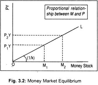
For equilibrium in the money market, = kPY … (3.12)

Equation (3.12) shows a proportional relationship between money stock and the price level. The quantity theory of money says that the quantity of money determines the price level. It is to be remembered here that Y is also fixed due to the existence of full employment in the economy.

Fig. 3.2 represents money market equi­librium where we plot total money stock M on the horizontal axis and the levels of PY on the vertical axis. The vector (OL), the slope of which is (1/k), shows the levels of PY that can be supported by different quantities of money supply. As money supply increases from M₁ to M₂, the price level rises proportionately from P₁to P₂.

Thus, we see a link between money supply and the price level: an excess money supply means increasing demand for commodities that pulls up the general price level. But money supply does not have any impact on Y which is determined in the real sector and Y is fixed due to full employment. The only way for equilibrium output to change in this classical model can be attributed to a shift in labour demand or labour supply curve.

One essential feature that follows from the classical money market is that money is neutral. This means that changes in money stock affect only absolute prices and money wages proportionately. Real variables such as, output, level of employment and real wage rate remain undisturbed following a change in money supply.

3. Interest Rate Determination: Goods Market:

In the classical model the components of aggregate demand consumption and investment determine equilibrium interest rate. Interest rate that guarantees that changes in the particular components of demands do not affect the aggregate level of commodity demand. It may be noted here that the interest rate is a ‘real’ variable in the goods market. The goods market is concerned with the way the fixed output or income is split between saving and consumption. Here we determine equilibrium rate of interest.

Saving implies a choice between present and future consumption. People save in the current period to have larger income or consumption at a future date. Of course, such saving then depends on the rate of interest in the classical system, and not on income as was said by J. M. Keynes.

Classicists assumed that saving (S) is an increasing function of the rate of interest (r), that is,

S = f (r) …..(3.13)

Investment may be defined as the amount of an economy’s product that is not consumed. Investment refers to the creation of additional stock of capital. An investment is something that is used to create value in future. An economy considers a number of capital projects in each time period. It undertakes those investment projects that yield a rate of return greater than the market rate of interest. Thus, investment, in the classical system, depends on the market rate of interest.

Investment is an inverse function of the rate of interest, that is,

I = f(r) ………(3.14)

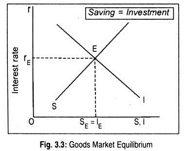
The goods market equilibrium is achieved when saving is equal to investment, i.e.,

S = I ………..(3.15)

A flexible interest rate in the classical system always brings equality between savings and investment. Fig. 3.3 shows how equilibrium rate of interest is determined in the classical model, independent of the monetary sector. Saving curve (S) and investment curve (I) are equal to each other at point E where the equilibrium volume of saving (S_E) is equal to the equilibrium value of investment (I_E). Interest rate is flexible and it adjusts to maintain the equality between saving and investment. The equilibrium interest rate is a real variable and in no way influenced by the quantity of money.

1. Classical Dichotomy:

One important conclusion from the classical model is the classical dichotomy. Quantity of money does not influence the real variables of the system- output, employment, and the interest rate. Quantity of money only influences the price level. This means that the goods market is segmented completely from the remainder of the system. Real sectors cannot influence the monetary sector and, hence, monetary variables. Monetary sector is not concerned with relative prices and real variables.

2. Policy Implications:

The policy implication of this classical model is that monetary policy alone can influence economic activity. What is required for stable price level is the stable money supply since quantity of money determines the price level. Fiscal policy is an impotent instrument to influence aggregate demand.