Purchase Plan of Consumers: 3 Effects | Economics

Given the consumer’s preference-indifference pattern, his equilibrium purchase plan would change if there is a change in his price-income situation. Here we have to consider three types of effect upon the purchase plan of the consumer. These are the income effect, the substitution effect and the price effect.

Effect # 1. The Income Effect:

Income effect is defined as the effect upon the purchase plan of the consumer of a change in his money income, the prices of the goods he buys remaining unchanged. Since a change in the money income of the consumer, the prices remaining constant implies a change in real income, the income effect actually is the effect of a change in the real income of the consumer.

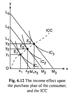
The income effect can be illustrated with the help of Fig. 6.12, where it has been assumed that the two goods that the consumer purchases and consumes are X and Y.

In Fig. 6.12, initially, the budget line of the consumer has been assumed to be L₁M₁. Subject to this budget line, the consumer’s equilibrium point has been obtained to be E₁(x₁,y₁) where the budget line L₁M₁ has touched one of his ICs, viz., IC₁. Now suppose, the consumer’s money income increases, the prices of goods X and Y remaining unchanged.

As a result, his budget line would have a parallel rightward shift from L₁M₁ to L₂M₂, say. The consumer’s equilibrium point on the new budget line will be the point E₂(x₂, y₂) which is also a point on IC₂.

That is, as a result of an increase in the consumer’s money income, the prices of the goods remaining constant, his equilibrium point and purchase plan would move from the point E₁(x₁, y₁) on IC₁ to the point E₂(x₂, y₂) on a higher IC, IC₂.

This movement in his equilibrium point and this change in his purchase plan represent the income effect. That the consumer has now moved on to a higher IC indicates that his real income has increased.

In Fig. 6.12, it is seen that when the money income of the consumer rises, the prices remaining constant, his purchase of both the goods increases. 

It all depends on the shape of his ICs, i.e., on his preference-indifference pattern. But it should be remembered that as his money income rises, the consumer must purchase at least one of the goods in a larger quantity, because it is assumed that the utility-maximising consumer spends all his income on two MIB goods. If he buys both the goods in a smaller quantity, he would not be able to spend all his income.

The Income-Consumption Curve:

Now suppose, the consumer’s money income increases further and his budget gets a parallel shift again from L₂M₂ to L₃M₃ in Fig. 6.12. As a result, his equilibrium point would move from the point E₂ (x₂, y₂) to the point E₃ (x₃, y₃) on a higher IC, viz., IC₃.

In the analysis, the consumer’s money income increases, the prices remaining constant, his equilibrium point moves from the point E₁ to E₂ to E₃, and so on. Now join these equilibrium points and the point of origin O, it is known as the consumer’s income-consumption curve (ICC).

This curve is shown to be the curve OE₁E₂E₃ … in Fig. 6.12. The ICC has been made to start from the point of origin or rather, looking at it from the opposite direction, it has been made to come to an end at the origin, because in the event of successive income decreases, the equilibrium point of the consumer would move from the point, say, E₃ to E₂ to E₁ to.,. along the ICC.

So if the income goes on decreasing indefinitely, the consumer’s equilibrium point would be approaching the point 0(0, 0).

A formal definition of the ICC may be given in this way:

An income-consumption curve is one that starts from the origin and passes through the successive equilibrium points of the consumer that are obtained as a result of successive increases in his money income, the prices of the goods remaining constant.

Superior Goods, Normal Goods and Inferior Goods:

Usually, when the consumer’s money income rises, the prices of the goods remaining constant, i.e., when his real income rises, relative prices remaining the same, i.e., when his budget line gets an upward parallel shift, he would buy more of both the goods.

If, as a result of a 1 per cent rise in the consumer’s money income, his purchase of any good X increases by more than 1 per cent, i.e., if the coefficient of his income-elasticity of demand for X (η_x) is greater than one (η_x > 1) then the good is called a superior good, where η_x is

On the other hand, if as a result of a rise in consumer’s income by 1 per cent, his demand for X remains the same, or, if it rises by less than or equal to 1 per cent, then the good is called a normal good.

That is, in the case of a normal good 

0 ≤ η_X< 1.

Lastly, if as a result of a rise in consumer’s income, his demand for any good, X, falls, then the good is called an inferior good.

In the case of an inferior good, then:

η_x< 0. (6.37)

It may be noted here that in this two-commodity indifference curve analysis, both the goods may be non-inferior, but only one of them can be inferior. This is because if his money income rises, prices remaining constant, he may buy more of both the goods or, less of one good and more of the other, thereby spending all his money and keeping himself on the (new) budget line at the point of tangency.

On the other hand, if he buys less of both the goods as his money income rises, prices remaining constant, he would not spend all his money income—he would move to a point on a lower IC to the left of the budget line. This is contrary to the assumption of utility-maximisation.

Therefore, in the case of a normal or a superior good, a rise (fall) in the money income of the consumer would result in its demand remaining the same or rising (falling) is obtained. On the other hand, in the case of an inferior good, a rise (fall) in his money income would result in a fall (rise) in his demand for the good.

Effect # 2. The Substitution Effect—Hicks and Slutsky:

The Hicks-SE:

The substitution effect (SE) upon the purchase plan of the consumer is the effect of a change in the relative prices of the goods that he purchases (here good X and good Y), his real income remaining constant.

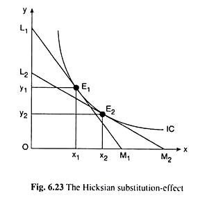
Real income has to remain constant because, if there is any change in real income, then the substitution- and income effects would get mixed up. First let’s explain the SE following Hicks, the Hicksian SE, so to say, with the help of Fig. 6.23.

In Fig. 6.23, initially, the budget line of the consumer is L₁M₁, and his equilibrium point is E₁ on the indifference curve, IC₁. At E₁ he purchases the commodity combination E₁ (x₁ y₁). Now, if the price of good X diminishes, his money income and the price of Y remaining the same, the consumer’s real income would increase.

In order to keep his real income unchanged at the initial level, let us increase the price of Y ‘appropriately’. Now, since the price of X has decreased and the price of Y has increased appropriately, the relative prices of the goods have changed—X has become relatively cheaper and Y has become relatively dearer—the consumer’s real income remaining constant.

His budget line would now become flatter, because its x- intercept would increase and y-intercept would decrease and the new budget line, L₂M₂, would touch the same IC, viz., IC₁, at the point E₂, i.e., the consumer now would be in equilibrium at the point E₂ (x₂, y₂).

The movement of his equilibrium point from E₁ to E₂ along the same IC, viz., IC₁, gives us the effect of a change in the relative prices of the goods, his real income remaining constant.

That is, this movement represents the SE. Owing to the SE, the consumer would purchase the relatively cheaper good X in a larger quantity—this quantity would increase from x₁ to x₂, and he would purchase the relatively dearer good Y in a smaller quantity—this quantity would fall from y, to y₂. In other words, owing to the SE, the consumer would substitute the relatively cheaper commodity for the relatively dearer one.

If, initially, the budget line of the consumer and his equilibrium point are L₂M₂ and E₂ (x₂, y₂), respectively, and if, now, the price of X increases and price of Y diminishes appropriately so that the real income of the consumer remains constant, then his budget line would become steeper—it would be, say, L₁M₁—and his equilibrium point now would be E₁ (x₁, y₁,).

The consumer now, as before would buy the relatively cheaper commodity Y in a larger quantity (from y₂ to y₁) and the relatively dearer commodity X in a smaller quantity (from x₂ to x₁), i.e., here again, he would substitute the relatively cheaper good for the relatively dearer good.

The Slutsky-SE:

According to Slutsky also, SE is the effect of a change in the relative prices of the goods, the consumer’s real income remaining constant. But the Hicks-SE and the Slutsky-SE are different because their interpretation of constancy of real income is different. According to Hicks, real income means the level of satisfaction.

Here real income remains constant means the level of satisfaction remains constant, i.e., the consumer remains on the same IC. According to Slutsky, on the other hand, real income remains the same means the consumer has at least the purchasing power to have the initial equilibrium combination of goods.

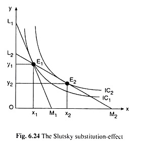
Therefore, the Slutsky-SE is obtained if the relative prices of the goods change, the consumer’s purchasing power to obtain the initial equilibrium combination of goods remaining intact. The Slutsky-SE can be illustrated with the help of Fig. 6.24.

 

In Fig, 6.24, initially, the budget line and the equilibrium point of the consumer are L₁M₁ and E₁(x₁, y₁,) respectively. Now suppose, the price of X falls and price of Y rises, the consumer’s real income in the Slutsky sense, remaining constant.

The new budget line, L₂M₂, then would be flatter than L₁M₁, (since its numerical slope, p_x/p_Y has diminished) and it would pass through the point E₁(x₁, y₁,). That the budget line, L₂M₂, passes through the point E₁(x₁, y₁,) implies that in the new situation also he can buy the initial equilibrium combination (x₁, y₁) if he wishes.

The utility-maximising consumer, however, would not buy at the point E, on the budget line L₂M₂. He would be in equilibrium at the point of tangency E₂(x₂, y₂) between the budget line L₂M₂ and the indifference curve IC₂. Therefore, the movement in his equilibrium point from E₁(x₁ y₁,) to E₂(x₂, y₂) represents the Slutsky-SE.

Because of the Slutsky-SE also, the consumer would buy the relatively cheaper commodity X in a larger quantity (x₂ > x₁) and the relatively dearer commodity Y in a smaller quantity (y₂ < y₁), i.e., he would substitute the relatively cheaper good for the relatively dearer good. However, there is an important difference between the Hicks and Slutsky SEs.

In the case of the former the consumer remains on the same IC (viz., IC₁) as in the initial position. But in the latter case, the consumer moves from a lower IC, viz., IC₁, to a higher IC, viz., IC₂. This difference is due to the difference in the idea of constancy of real income in the two cases. Since the Slutsky SE takes the consumer to a higher IC, it is considered as under-compensatory.

Substitution Effect and the Convexity of the ICs:

Owing to the SE, the consumer would buy the relatively cheaper good in a larger quantity and the dearer good in a smaller quantity. This will be obtained, because of the convexity of the ICs.

Initially, the consumer is in equilibrium at the point E₁ on IC₁ in Fig. 6.23. As the price of good X falls and the price of good Y rises, the consumer’s budget line would become flatter. In the Hicks case, the flatter budget line would touch the same IC (IC₁) at a point E₂ where the IC also is flatter.

Since the IC is convex to the origin, it is flatter downwards to the right. That is, the flatter budget line would touch the same IC at a point which is downward towards right of the initial equilibrium point. That is why the consumer’s purchase of X would increase (from x₁ to x₂) and his purchase of Y would decrease (from y₁ to y₂).

Similarly, if the consumer’s initial budget line and equilibrium point are L₂M₂ and E₂(x₂, y₂) and if now p_x increases and p_v diminishes, real income remaining constant, his budget line would become steeper—it would be L₁M₁—and the steeper line would touch the same IC (IC₁) at a point E₁(x₁, y₁,) where the IC is steeper.

The point must lie upward towards left of the point E₂ because of convexity of the IC. Therefore, the consumer now would buy the relatively cheaper good Y more and the rela­tively dearer good X less.

Therefore, that the convexity of the ICs and whatever it stands for, the dimin­ishing MRS_X,_Y, etc., gives rise to the fact that the SE would make the consumer buy the rela­tively cheaper good more and the relatively dearer good less.

The same kind of reasoning also applies to the explanation of why owing to the Slutsky SE, the consumer substitutes the relatively cheaper good for the relatively dearer one.

Effect # 3. The Price Effect:

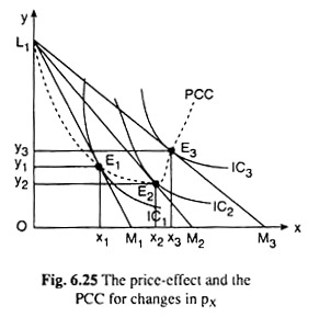
The price effect is the effect upon the purchase plan of a consumer, of a change in the price of one of the goods, the price of the other goods and his money income remaining unchanged. Let’s explain this effect with the help of Fig. 6.25 where the consumer has been assumed to purchase only two goods, X and Y.

In Fig. 6.25, let us suppose that, initially, the budget line and the equilibrium point of the consumer are L₁M₁ and E₁ (x_1,y₁) on IQ, respectively.Now suppose, the price of good X falls, the price of good Y and the money income of the consumer (i.e., the other things) remaining the same.

Consequently, his budget line L₁M₁ would rotate anticlockwise about the point, L₁ and it would be a line like L₁M₂. For, the x- intercept of the budget line (M/p_x) would now increase from OM₁ to, say, OM₂, and the y-intercept of the line (M/p_y)would remain the same.

It is seen in Fig. 6.25 that the new budget line L₁M₂ would touch a higher IC, IC₂, at the point E₂(x₂, y₂). That is, the consumer’s new equilibrium point would be E₂.

This movement in his equilibrium point from E₁ on IC₁ to E₂ on IC₂ is caused by the ceteris paribus change in p_x, and it represents the price effect (PE). As a result of the PE, the consumer’s purchase of X would rise from x₁ to x₂ and his purchase of Y would fall from y₁ to y₂.

 

Also, owing to the PE, the consumer’s level of satisfaction rises as his equilibrium point shifts from E₁ on IC₁ to E₂ on a higher IC, viz., IC₂. This rise in his level of satisfaction is obtained as his real income level has increased because of a fall in p_x, p_y and M remaining constant.

As the price of good X changes, what happens to the quantity demanded of X, is of much interest to us. Incidentally, it can also be seen what happens to the demand for the other good, Y.

The Price-Consumption Curve:

In Fig. 6.25, initially, the consumer’s budget line and his equilibrium point are L₁M₁ and E₁ (x_1,y₁) on IC₁. It is also seen that as p_x diminishes, ceteris paribus, the consumer’s equilibrium point moves from E₁ (x₁, y₁) on IC₁ to E₂(x₂, y₂) on a higher IC, viz., IC₂.

If, now, p_x diminishes again, other things remaining the same, his budget line would rotate from L₁M₂ to L₁M₃ and his equilibrium would be established at a point like E₃(x₃, y₃) on a still higher IC, viz., IC₃, and the process would go on like this.

Now join the points L₁ and the successive equilibrium points of the consumer E₁ E₂, E₃,…, obtained as a result of successive falls in p_x, other things remaining constant, by a curve, it is called the price-consumption curve (PCC).

It follows that every point on the PCC is an equilibrium point of the consumer. It may be noted that L₁ has been taken to be a point on the PCC because it is the limiting point to which the equilibrium point of the consumer would approach as the price of good X increases indefinitely, other things remaining the same.

For example, suppose, the initial equilibrium point is E₃. Now, as p_x increases indefinitely, the budget line of the consumer would become steeper and his equilibrium point would move along the PCC from E₃ to E₂ to and so on, and the consumer’s purchase of X diminishes and tends to zero and his purchase of Y increases and tends to OL₁ i.e., the consumer’s equilibrium combination would approach the point L₁(0, OL₁), and his budget line would tend to become the vertical line OL₁.

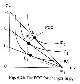
In Fig. 6.25, the PCC obtained is for changes in the price of good X. Let’s now obtain the PCC for changes in the price of good Y. In Fig, 6.26, L₁M₁ is the consumer’s initial budget line and E₁ is his initial equilibrium point. Now suppose that p_Y diminishes, p_x and M remaining constant.

Consequently, the budget line of the consumer would rotate clockwise about the point M₁ to become a line like L₂M₁ for, now the x-intercept of the line (M/p_x) would remain the same and the y-intercept (M/p_Y) would increase. As a result, his equilibrium point would move from the point E₁ on IC₁ to E₂ on a higher curve, IC₂.

The equilibrium point moves to a higher IC because the real income of the consumer has increased on account of a ceteris paribus fall in p_Y. The movement in the consumer’s equilibrium point from E, to E₂ represents the price-effect of a change (fall) in p_Y. Due to the PE, the consumer’s purchase of Y has increased and his purchase of X has decreased.

To obtain the PCC for changes in p_Y, now suppose that p_Y diminishes again. As a consequence, the consumer’s budget line would become L₃M₁ and his equilibrium point would move from the point E₂ on IC₂ to E₃ on a higher curve, IC₃, and the process would go on as p_Y falls again and again. Now join the points M₁ and the equilibrium points E₁, E₂, E₃,…, it may be called the PCC for changes in p_Y.

Note that like L₁ in the earlier case, the point M₁ has been taken to be a point on the PCC in Fig. 6.26. This is because M₁ is the limiting position of the consumer’s equilibrium point as p_Y rises.

As p_Y rises indefinitely, the equilibrium point would be moving from … to E₃ to E₂ to E₁ and so on, and the consumer’s purchase of Y would diminish and tend to zero and his purchase of X would increase and tend to become equal to OM₁ i.e., the consumer’s equi­librium combination would approach the point M₁(OM₁, 0), and his budget line would tend to become the horizontal line OM₁.