The Theory of Market Demand (Recent Developments)

A. The Pragmatic Approach to Demand Analysis:

Many writers have questioned the usefulness of the various theories of consumers’ behaviour.

There has been an increasing awareness that although the various approaches to utility are theoretically impressive, there is very little an applied economist can use to explain the complexity of the real world.

Thus many writers have followed a pragmatic approach to the theory of demand.

They accepted the fundamental ‘law of demand’ on trust, and formulated demand functions directly on the basis of market data without reference to the theory of utility and the behaviour of the individual consumer. Demand is expressed as a multivariate function, and is estimated with various econometric methods.

Such demand functions refer obviously to the market behaviour of the con­sumers, that is, to the behaviour of all consumers as a group, and not to the behaviour of single individuals. Furthermore, in most cases the demand functions refer to a group of commodities, e.g. demand for food, demand for consumer durables, etc.

Serious difficulties arise in estimating demand functions. The aggregation of demand over individuals and over commodities makes the use of index numbers inevitable, but the problems associated with such indexes are numerous. Furthermore, there are various other estimation problems which impair the reliability of the statistically-estimated demand functions.

The most important of these difficulties arise from the simultaneous change of all the determinants, which makes it extremely difficult to assess the influence of each individual factor separately. However, there has been a continuous improve­ment in the econometric techniques and currently demand functions are fairly easy to estimate statistically.

The constant-elasticity demand function:

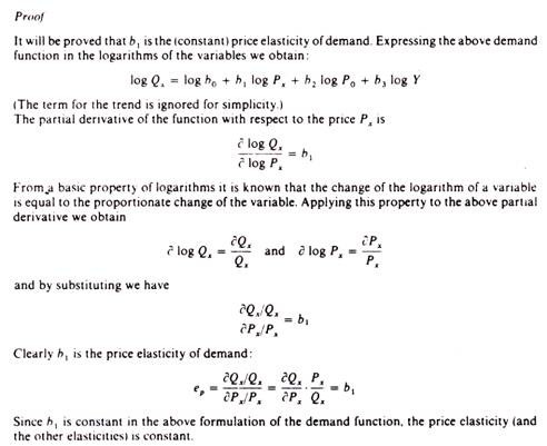
The most commonly used form of demand function in applied research has been the ‘constant-elasticity’ type:

Q_x = b₀ – P^b_x¹. P^b₀². Y^b3. e^b4t

Where Q_x = quantity demanded of commodity x

P_x = price of x

P₀ = prices of other commodities

Y = consumers’ aggregate income

e^b4t = a trend factor for ‘tastes’ (e = base of natural logarithms)

b₁ = price elasticity of demand

b₂ = cross-elasticity of demand

b₃ = income elasticity of demand

The term ‘constant elasticity demand function’ is due to the fact that in this form the coefficients b₁, b₂, b₃ are elasticity’s of demand which are assumed to remain constant.

Usually the followers of the pragmatic approach, although not adhering to utility functions, express the demand function in such a way as to incorporate the assumption of ‘no money illusion’ postulated by the traditional theory of the consumer. In technical jargon they express the demand as a homogeneous function of degree zero. This has been (most commonly) effected by introducing real income and relative prices in the function, that is

where P is a general price index. In this formulation it is obvious that if prices and income change by the same proportion, for example by k per cent, the quantity demanded of x will not change, because k will appear in both the numerator and the denominator of the relative prices and real income, and hence will cancel out. The new quantity demanded will be the same as the initial one: there is no money illusion in the behaviour of the consumer.

Dynamic versions of demand functions: Distributed-lag models of demand:

A recent development in demand studies is the expression of demand functions in dynamic form.

Dynamic demand functions include lagged values of the quantity demanded and of income as separate variables influencing the demand in any particular period. Dynamisation of the demand functions expresses the generally accepted idea that current pur­chasing decisions are influenced by past behaviour.

To express the idea that current decisions are influenced by past behaviour we must postulate a particular type of relationship between the past and the present. The most common assumption in this respect is that current behaviour depends on past levels of income and past levels of demand. If the commodity is a durable past purchases con­stitute a ‘stock’ of this commodity which clearly affects the current (and future) purchases of such durable.

If the commodity is non-durable (for example, tobacco, food, etc.), past purchases reflect a habit which is acquired by buying and consuming the commodity in the past, so that the level of purchases in previous periods influences the current (and future) patterns of demand. Incorporating the influence of past decisions and experiences in the demand function is a way for rendering it dynamic.

Another usual assumption concerning the way in which past behaviour affects the present is that the more recent of past levels of income or demand have a greater influence on present consumption patterns than the more remote ones (for example, we are more influenced by our income in the last year than by the income we earned five or ten years ago).

Models (functions), including lagged values of demand, of income (or of other vari­ables) are called distributed-lag models’. In general form a distributed-lag model may be expressed as

The number of lags depends on the particular relationship being studied. The necessity of a dynamic approach has long been recognized for the study of the de­mand of certain commodities (consumer durables). R. Stone extended the dynamic formulation to a wider range of commodities. Houthakker and Taylor’ generalized the dynamisation of demand functions.

A widely used model, both in demand functions and in investment functions, is the model based on the ‘stock-adjustment principle’, which has been developed by Nerlove. This model has initially been applied to the study of demand functions for consumer dur­ables. Recently Houthakker and Taylor have extended the ‘stock-adjustment principle’ to non-durables, giving it the name ‘habit-creation principle’.

Nerlove’s ‘stock-adjustment principle’:

The model as applied to consumer durables re­sults in a demand function of the form

Q_(t) = a₁ Y_(t) + a2 Q_{(t – 1)}

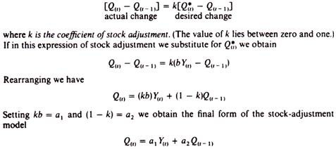
The model is derived as follows. There is a desired level of durables Q*_(t), which is deter­mined by the current level of income:

Q*_(t) = b Y_(t)

However, the consumer cannot immediately acquire the desired level of durables due to limited income, credit limitations, etc. Thus in each period the consumer acquires only a part of the desired level. In other words, the acquisition of the desired level of durables is gradual; in each period we come closer to Q*_(t).

In each period we purchase a certain quantity Q_(t). There is an actual change from the quantity bought in the previous period denoted by the difference Q_(t) – Q_{(t – 1)}. This change in actual purchases is only a fraction k of the desired change, Q*_(t) – Q_{(t – 1)}. Thus

Houthakker’s and Taylor’s dynamic model:

Their model is based on Nerlove’s formul­ation. They extended the idea of stock adjustment to non-durables. The current demand for durables depends on, among other things, the stock of such commodities (stock- adjustment process). The current demand for non-durables depends on, among other things, the purchases of the commodities in the past, because by consuming a certain commodity we get accustomed to it (habit-formation process). The demand function is of the form

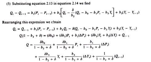
where ΔY_t is the change in income and ΔP_t is the change in price between period t and t — 1. The demand function is derived as follows.

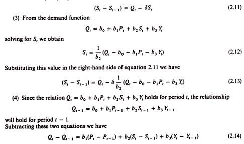
Demand in any particular period depends on price, on stocks of the commodity and on the current level of income

Q₁ = b₀ + b₁P_t + b₂S_t + b₃Y_t (2.10)

Where S_t = stocks of durables, if the function refers to such goods

S_t = ‘stocks of habits’, if the function refers to non-durables

The sign of the coefficient of S will be negative for durables: the more we have of furniture, electrical appliances, etc., the less our demand for such commodities will be.

The sign of the coefficient of S will be positive for non-durables the higher our pur­chases of non-durables the stronger our habit becomes.

Stocks S, however, cannot be measured:

(i) The stock of durables is composed of heterogeneous items of various ages-the electrical equipment we have is not of the same age, some items may be very old and need scrapping and replacing, some others are new. Their heterogeneity also makes direct measurement difficult. What we ideally want for stocks is the sum of depreciated inventories of durables; but the appropriate deprecia­tion rates are not known.

(ii) The ‘stock of habits’ is a psychological variable and cannot be quantified.

However, we can eliminate algebraically stocks, S_t, from the demand function and replace it with other measurable variables by making some ‘reasonable’ assumptions.

For durables the elimination process may be outlined as follows:

(1) The net change in stocks realized in any period (S_t – S_t-1) is equal to our purchases in that period minus the depreciation of our old possessions

S_t – S_t-1 = Q_t – depreciation

(2) Assume that depreciation is equal in all the periods of the life of the durable, i.e.,

Depreciation = δS_t

Where δ is a constant depreciation rate (for example, if the life of the durable is ten years, we assume that the yearly depreciation is 10 per cent of the value of the durable). Thus

Setting a₀, a₁, a₂, a₃, a₄ and a₅ for the coefficients of this equation we arrive at the final form of Houthakker’s and Taylor’s formulation

Q_t = a₀ + a₁p_t + a₂(ΔP_t) + a₃ Y_t + a₄(ΔY_t) + a₅Q_{t – 1}

B. Linear Expenditure Systems:

These are models which deal with groups of commodities rather than individual commodities. Such groups, when added, yield total consumer expenditure. Linear expenditure systems are thus of great interest in aggregate econometric models, where they provide desirable disaggregation of the consumption function. One of the earliest linear expenditure models was suggested by R. Stone (Economic Journal, 1954).

The linear expenditure systems (LES) are usually formulated on the basis of a utility function, from which demand functions are derived in the normal way (by maximization of the utility function subject to a budget constraint). In this respect the approach of LES is the same as that of models based on indifference curves.

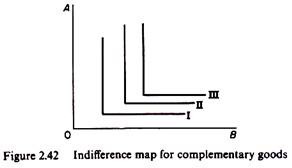
However, LES differ in that they are applied to ‘groups of commodities’ between which no substitution is possible, while the indifference-curves approach is basically designed for handling commodities which are substitutes. The very notion of an indifference curve is the substitutability of the commodities concerned. Actually the indifference map of a LES would appear as in figure 2.42, implying the non-substitutability of groups of commodities.

The utility function is additive, that is, total utility (U) is the sum of the utilities derived from the various groups of commodities.

For example, assume that all the commodities bought by the consumers are grouped in five categories:

A Food and beverages

B Clothing

C Consumers’ durables

D Household-operation expenses

E Services (transport, entertainment, etc.).

The total utility is

U = ∑ U_i

or

U = U_(A) + U_(B) + U_(C) + U_(D) + U_(E)

Additively implies that the utilities of the various groups are independent, that is, that there is no possibility of substitution (or complementarity) between the groups A, B, C, D and E. In linear expenditure systems the commodities bought by the consumers are grouped in broad categories, so as to be compatible with the additively postulate of the utility function. Thus each group must include all substitutes, and complements. In this way substitution between groups is ruled out, but substitution can occur within each group.

The consumers buy some minimum quantity from each group, irrespective of prices. The minimum quantities are called ‘subsistence quantities’ because they are the minimum requirements for keeping the consumer alive. The income left (after the expenditure on the minimum quantities is covered) is allocated among the various groups on the basis of prices.

The income of the consumer is, therefore, split into two parts the ‘subsistence income’, which is spent for the acquisition of the minimum quantities of the various commodities, and the ‘supernumerary income’, the income left after the minimum expenditures are covered.

A simple linear expenditure system:

The utility function may take any additive form.

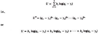
Stone’s utility function, for example, is additive in the logarithms of the group utilities:

Where y_i, = minimum quantity of group i

b_i = marginal budget shares; that is, each b_i shows by how much the expenditure on group i will increase if total income changes by one unit (see below)

It is assumed that the total income is spent (budget constraint). Hence ∑ b_i = 1, since the changes of expenditures must be equal to the change in income (by the budget constraint).

Other crucial assumptions of this model are:

(1) Rationality of the consumers

(2) Additively of utilities

(3) 0 < b, < 1

Y_i > 0 (there is no negative minimum quantity)

(q_i – y_i) > 0 (some quantity above the minimum is purchased)

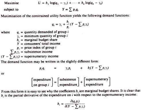
The consumers maximize their total utility, subject to the (total) income constraint.

In the case of Stone’s utility function we have:

There are various versions of the linear expenditure model, depending on the form of the utility function. Various writers assume a different form of the utility function and hence they derive a different formulation of the demand functions.