Indifference-Curves Analysis (With Diagram)

1. The leisure-income trade-off and the need for overtime rates higher than the normal wage rate:

Indifference-curves analysis may be used to explain why firms must pay higher rates for overtime work.

We first derive the income-leisure curve of an individual consumer. This curve shows different combinations of income, earned by working, and leisure time.

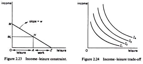
Assume that we measure money income on the vertical axis and leisure time on the horizontal axis. Assume further that the maximum time available for either leisure or work is 0Z hours a day.

The individual can either use all the 0Z hours for leisure, in which case he earns zero income, or he can choose to work all the 0Z hours and earn a maximum money income 0M (given the current market wage rate w) or he can use part of the 0Z hours for leisure (e.g. 0A) and the remaining (AZ) hours for work, in which case he would earn 0M₁ income.

The line MZ is the income-leisure curve, which shows how much time of his leisure an individual must give up if he wants to earn a certain income.

The slope of the income-leisure line is equal to the market wage rate.

We may next construct the indifference map of the individual, which shows the ranking of his preferences as between income and leisure. Each indifference curve shows various combinations of income and leisure which yield the same level of satisfaction (utility) to the individual. The indifference curves have the usual properties they are convex to the origin, they do not intersect and they show a higher level of satisfaction the further away from the origin they are.

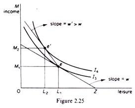
The individual’s equilibrium is determined by the point of tangency of his income- leisure line with the highest possible trade-off curve (point e in figure 2.25). Given the wage rate w, the individual maximizes his utility by working L₁Z hours, earning income 0M₁, and using the remaining time (0L₁) for leisure.

If firms want more hours of work they will have to pay a higher hourly rate than the normal w in order to give an incentive to the individual to reduce his leisure time. An increase in the overtime rate is depicted by a leisure-income line which is steeper to the left of e (figure 2.25). With higher overtime payment the individual will be induced to give up some of his leisure time because in this way he will reach a higher indifference curve. The income-leisure line becomes kinked at e, and the new equilibrium of the individual is at e’ on indifference curve I₄, showing that he will increase his working hour (by L₁L₂) and earn a higher income (0M₂ > 0M₁).

2. Evaluation of alternative government policies using indifference-curves analysis:

Indifference curves may be used to evaluate the effects of alternative government policies. For example, assume that the government considers either the adoption of a food subsidization policy for pensioners or granting a supplementary income to them. Which of these measures costs less to the government (and hence to the tax payer)? What are the effects of these policies on the demand patterns of a pensioner? Such questions may be answered by using indifference-curves analysis. We will illustrate the way in which the above information may be obtained, assuming for simplicity that there is a single pensioner and two commodities, x (food) and y (money income).

The initial equilibrium of the pensioner is at point e_i, where his budget line, AB, is tangent to indifference curve I₁ he consumes 0X_1; units of food, paying ZA of his income, and having 0Z income left over to spend on other commodities. The goal of the government is to make it possible for the pensioner to move to the higher level of welfare (satisfaction) denoted by the indifference curve I₂.

The effects of the food subsidy:

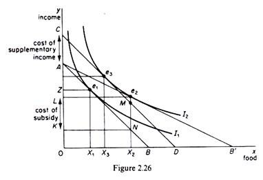
Assume that the government gives food coupons to the pensioner which allow him to buy food at half the market price. Following this measure the budget line of the pensioner shifts to AB’, which is tangent to I₂ at point e₂. At his new equilibrium position the pensioner buys 0X₂ units of food, paying for this quantity AL of his income. If there were no food subsidy the pensioner would have to spend AK of his income to buy 0X₂ units of food.

Since he pays only AL, the difference LK – (AK — AL) must be paid to the food producers by the government.

Thus, if the govern­ment adopts the food subsidy policy we have the following effects:

(a) The cost to the government (and to the taxpayer) is LK.

(b) The market price of food is not affected by this policy, so that other consumers continue to pay the original price,

(c) The govern­ment is certain that the pensioners will consume more food.

This effect may be partic­ularly desirable (as a subsidiary goal of the government) if there are surpluses of food. Actually it is often the case that food subsidies are designed in such a way as to benefit not only the consumers but also the producers of foodstuff, (d) the assistance to pen­sioners via the food subsidy imposes a certain pattern of consumption, a certain choice of spending their income.

The effects of a supplementary income policy:

Assume that the government considers granting to the pensioner a supplementary income which will enable him to reach the higher welfare level implied by indifference curve I₂. To find the amount of such a supplementary income we simply draw a budget line (CD), parallel to the original budget line (AB) and tangent to I₂ (at point e₃). The pensioner will now buy 0X₃ units of food. The cost to the government of the supplementary income policy is equal to CA, which (in our example) is smaller than the cost of the food subsidy policy. Furthermore the quantity of food in this case (0X₃) is smaller than the quantity which would be bought under a food subsidy programme (0X₂).

Comparing the two alternative policies we observe that both policies achieve the government’s goal of enabling the pensioner to reach the higher welfare state implied by I₂. But the food subsidy programme is more costly (in our example) than the supple­mentary income policy. In fact if the government were to give to the pensioner the cost of the subsidy in the form of supplementary income, the pensioner would attain a higher level of satisfaction (an indifference curve above I₂). However, the consumption of food will be greater in the case of the food subsidy policy.

Which one of these alternative policies the government will adopt depends not only on the above considerations, but also on the other goals of the government and the indirect effects of each policy. For example, if there is a surplus food production, the government may adopt the more costly subsidization policy, which, apart from increas­ing the welfare of the consumer, also benefits the producers by reducing or even elimina­ting the surplus. Furthermore, supplementary incomes policies are in general more inflationary than price subsidies to specific individuals (especially if there is a surplus of the subsidized commodities). Increasing the incomes of some groups of ‘needy’ consumers may lead to increases of the market prices of commodities for all consumers, thus decreasing their welfare. The above discussion illustrates how indifference-curves analysis may give insight into, the implications of selective government measures, and thus help efficient policy formulation.

3. Indifference-curve analysis and the theory of exchange:

Indifference-curves analysis may be used to explain why exchange of commodities among individuals (or groups of individuals, countries, regions, and so on) takes place. We will show that, under certain conditions, exchange of commodities leads to an increase in the welfare of at least one individual without any reduction in the welfare of the other, so that the overall welfare which can be enjoyed from a given bundle of commodities is increased.

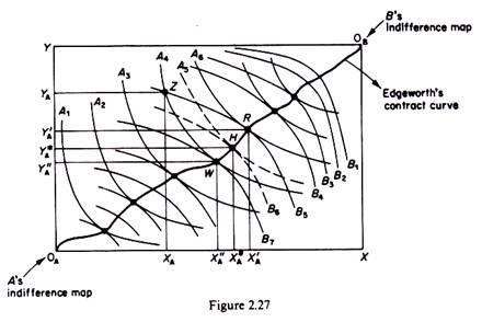
We will use the device of the Edge-worth box. We assume that there are only two individuals, A and B, and two commodities, x and y, whose quantities are given. These quantities are measured along the sides of the Edge-worth box. Any point of the Edge- worth box shows a certain distribution of the available quantities of x and y between individuals A and B.

The preferences of consumer A are represented by a set of indifference curves (denoted by A with an appropriate subscript) which are convex to the origin 0_A. The preferences of consumer B are represented by the set of indifference curves (denoted by B with an appropriate subscript) which are convex to 0_B. The indifference maps have the usual properties.

For example, the further down an indifference curve of B lies, the greater is the satisfaction. The two sets of indifference curves, being of opposite curvature, have points of tangency which form the so-called Edge-worth’s contract curve (0_A0_B in figure 2.27).

In other words the contract curve is the locus of points of tangency of the indif­ference curves of A and B, and therefore the locus of points at which the MRS of the two commodities is the same for both consumers

MRS^A_y,X = MRS^B_{y, x}

Only points lying on the contract curve represent optimal distribution of the avail­able quantities of x and y between the two consumers, in the sense that any diver­gence from this curve implies a lower level of satisfaction for at least one individual. For example, consider point Z off the contract curve. At this point consumer A owns 0X_A of commodity x and 0Y_A of commodity y, with the remaining quantities (X_AX and Y_AY) owned by consumer B.

With this distribution of the two commodities consumer A is on indifference curve A₄ while consumer B is on indifference curve B₅. We will show that point Z represents a suboptimal distribution of x and y, because if A and B exchange some of the quantities of the two commodities so as to move to any point on the section WR of the contract curve at least one (and probably both) of them will be better off (on a higher indifference curve) without the other being worse off.

If the consumers exchange x for y so that they arrive at the distribution denoted by R (consumer A giving away Y_AY’_A of commodity y in exchange for X_AX’_A of commodity x), consumer A will reach a higher welfare situation (moving from indifference curve A₄ to the higher one A₆) while consumer B retains his initial level of satisfaction (both Z and R lying on the same indifference curve B₅).

If the consumers reach, via exchanging commodity x for y, to the distribution denoted by W the opposite situation will obtain: consumer A will retain his initial level of satis­faction (since Z and W lie on the initial indifference curve A₄) while consumer B will attain a higher indifference curve (B₇).

If the consumers reach any other distribution between W and R, e.g. the one denoted by H, they will both be better off, reaching higher indifference curves (A₅ and B₆ re­spectively) as compared to their initial positions at Z.

If exchange takes place who will benefit more, A or B? The answer to this question cannot be given on purely economic criteria. The final distribution of x and y and the ‘gains’ from the exchange of these commodities will largely depend on the bargaining skills and power of the two individuals. Usually the consumers will reach a point between W and R, both gaining some welfare in the process.

In summary the contract curve includes optimal allocation of the commodities, in the sense that if the individuals are at a point off this curve they will gain by moving to a point on it, since at least one (or both) of them will be better off without the other becoming worse off.

It is implicit in the above elementary analysis of exchange that the tastes of A and B do not change and that the quantities of the two commodities are given. If these assumptions hold, the result of the act of exchange may be different.

4. Indifference-curves analysis of the cost of living:

Indifference-curve analysis and the theory of revealed preference can be used to establish whether, over a period of time during which both money incomes and prices have been changing, the consumer is better or worse off. The assumption underlying the following discussion is that the consumer spends all his money income in all time periods, that is, he chooses a point on his budget line in any particular period.

In the initial (base) period the consumer’s income and expenditure is:

Y₀ = ∑ q₀p0

And in the current period

Y₁ = ∑q₁p₁

Assuming that both prices and money income changed between the base and the current periods, how can we decide whether the consumer is better off? To answer this question we require index numbers of income and prices. An index of income changes is given by the expression

I_Y = (Y_t / Y₀). 100

Where Y₀ = money income in the base period

Y_t = money income in the current period

The index number of the income in the base period is 100. If in period t the index number is 125 we conclude that money income has increased by 25 per cent in period t as com­pared with the base period.

Changes in the price level are measured by two traditional price indexes, the Laspeyres price index, defined by

L = (∑q₀p_t /∑q₀p₀) . 100

and the Paasche index, defined by

P = (∑q_tp_t / ∑q_tp_o)

Where q₀ = quantities of the commodities bought in the base period

p₀ = prices of the commodities in the base period

q_t — quantities of the commodities bought in period t

p_t = prices of the commodities in period t

Given the above index numbers we will prove that:

(i) The consumer is better off in period t as compared with the base period if the index number of income is greater than the Laspeyres price index, that is, if

(Y_t / Y_o). 100 > L

(ii) The consumer is worse off in period t as compared with the base period if the index number of income is smaller than the Paasche price index, that is, if

(Y_t / Y_o). 100 > P

The use of the Laspeyres price index. Assume that the initial income and expenditure of the consumer is

Yo = ∑ q_op_o

In period t prices have changed to p_t, and if we estimate the cost of the ‘basket q₀‘ at the new prices we find

∑q_op_t

If ∑ q_op_t < Y_t, the initial ‘basket q₀‘ is available to the consumer in the current price (and income) situation. That is, with his current income (Y_t) the consumer can still purchase the original basket of goods if he so wishes. If he actually makes this choice in period t then

∑q_op_o = ∑q_op_t = Y_t

and the consumer retains the same level of satisfaction in period t as in the base period (he remains on the same indifference curve). However, if the consumer chooses in period t another basket of goods q_t (while q₀ continues to be available) then two situa­tions may occur:

either ∑q_op_t < ∑q_tp_t …(2.2)

which implies that q₀ is below the new budget line of the consumer, who, buying q_t, is better off (because he can buy basket q, which was beyond his means in the base period)

or ∑q_op_t = ∑q_tp_t

which implies that both baskets are equally expensive (q₀ and q_t both lie on the new budget line), but the consumer reveals his preference for q_t presumably because q, gives him more satisfaction (lies on a higher indifference curve).

Dividing equation (2.2) through by ∑ q₀p₀ (the initial income) and multiplying by 100 we obtain

The left-hand side of this inequality is the Laspeyres price index, while the right-hand side is the income index number ∑ q_tp_t, being the current income and ∑ q₀p₀ being the income of the base period). Thus we may write

L < [Y_t / Y_o. 100]

Which shows that the consumer is better off if the Laspeyres price index is smaller than the income index? This conclusion may be illustrated diagrammatically by using indifference curves.

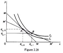
In figure 2.28 the initial budget line is MM, defined by the equation

Y₀ = ∑q₀p₀ = (q_x, ₀) (P_x.₀) + (q_y, ₀) (p_y, ₀)

The consumer is in equilibrium at point A, buying q_{x, 0} and q_{y, 0} of the two commodities.

The new budget line is M’M’ defined by the expression

Y_t = ∑q₁p_t = (q_{x, t}) (p_{x, t}) + (q_{y, t}) (p_{y, t})

The new budget line passes through the initial equilibrium point A, showing that ‘basket q₀‘ is still available to the consumer at the new set of prices (p_t). The consumer can, therefore, continue to purchase q₀, thus remaining on the initial indifference curve I₁. But he can reach a higher indifference curve (I₂) by choosing basket q_t shown by point B in figure 2.28.

This point was above the initial budget line, and hence beyond the reach of the consumer (given Y₀ and p₀). In other words the cost of bundle q_t (= point B) estimated at the original prices (p₀) was higher than the cost of bundle q₀ (at p₀). In the new price situation both bundles have the same cost since they lie on the new budget line (M’M’). Yet q_t is chosen because it lies on a higher indifference curve: the consumer is better off with the new income (Y_t) and the new set of prices (p_t).

The use of the Paasche price index. Assume, as before, that in the base period the con­sumer has income Y₀ and chooses basket q₀, spending on it all his income ∑ q₀p₀ = Y₀.

In the period t the consumer chooses a new basket q_t, spending all his income ∑q_tp_t = Y_t.

The cost of basket q_t, estimated at the prices of the base period, is ∑q_tp₀.

If ∑q₀p₀ > ∑q_tp₀ (2-3)

then the basket chosen in period t (q_t) was available in the base period, but was not chosen by the consumer, because presumably it was lying on a lower indifference curve than q₀.

Given that in period t the consumer does actually choose q_t spending all his income (∑q_tp_t) on it, it follows that basket q₀ is now beyond his means (i.e. q₀ is above the new budget line of the consumer). Hence the consumer is worse off in period t.

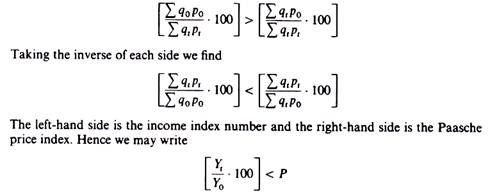
Dividing equation (2.3) through by ∑ q_tp_t and multiplying by 100 we obtain

that is, the consumer is worse off in period t as compared with the base period if the income index is smaller than the Paasche price index. We may show this result on a graph using indifference-curves analysis.

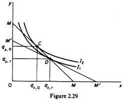
In figure 2.29 the equilibrium of the consumer in the base period is defined by C. Although basket D (including q_x, _t and q_y,_t) was on his original budget line, the consumer did not choose it, because it was lying on the lower indifference curve I₁.

In period t the new budget line (M’M’) defined by the expression

Y_t = ∑q_tp_t = (q_{x, t}) (p_{x, t}) + (q_{y, t}) (p_{y, t})

lies below basket q₀: the consumer cannot afford to buy the original bundle at the new prices (p_t). Thus the consumer chooses basket q_t, that is, he is worse off as compared to the base period. (If q₀ was available in period t and the consumer chose q_t, he would be inconsistent, since in the base period he had preferred q₀ to q_t).

It should be noted that comparisons of the above type are valid only if tastes and quality of the commodities have not changed in the two periods.