
The below mentioned article provides an overview on Supply.
Supply:
The quantity of a good or service offered for sale in a market depends on a large number of factors (variables). But, as in the case of demand, we ignore all of the relatively unimportant variables in order to concentrate upon those that have the greatest effect upon quantity supplied.
Certainly, the most important determinant of the quantity offered for sale is the price of the product under .consideration. The higher the price of the product, the more of it would be offered for sale.
Market Supply:
At any fixed point of time, there is also a definite relationship between the price of a good or service, and the quantity of it supplied. The supply relationship is ordinarily direct, which means that we expect quantity supplied to be greater at a higher price than at a lower price.
ADVERTISEMENTS:
A schedule that gives the quantities of a good or service supplied by all sellers at various prices is called a market supply schedule. Basically, a business firm is a producing unit that uses the services of labour, capital and natural resources to produce a saleable product.
A modern firm operating under a single management is assumed to extract the maximum amount of profit from the sale of its product. Given the costs of production for any given level of output, profitability is dependent on the price of the product. Profitability is also dependent on prices of other goods.
In any case, the market supply schedule is the aggregation of quantities that firms in an industry are willing to supply at various prices, and these firms are motivated by the criterion of profitability of their enterprise.
For example, an agricultural commodity such as wheat is produced by thousands of farmers in India. Whatever may be the state of technology (the amount of production), nature of the production process, quality of inputs (including fertility of the soil) we expect the quantity of wheat supplied to rise when the price of wheat rises.
ADVERTISEMENTS:
Given the costs of production and prices of other grains, we would expect more acres to be devoted to wheat when the price of wheat rises.
The reason is that the profitability of wheat has increased relative to other grains. This explains why cross elasticity of supply is more important than own price elasticity in case of two agricultural crops which compete for the same plot of land. We would expect acres to be diverted from wheat when the price of wheat falls. The reason is easy to find: the profitability of wheat has decreased relative to other grains.
In this way, it can be seen that acreage can be taken out of production of rice, oilseeds and soybeans and put into wheat. Or, in the later case, land can be diverted from wheat and put into other crops. It can be seen also that some farms are at the margin of profitable production at any given price.
If the price rises, such farms start production by joining the industry, but if the price falls, such farms essentially leave the industry.
ADVERTISEMENTS:
Managerial decisions on the level of wheat production have an impact on the quantities of wheat supplied, but decisions to enter or leave the wheat industry also have impact on them. These decisions are motivated by considerations of profitability, and profitability is partially dependent on the market price of wheat.
The market supply of wheat is, therefore, a schedule, that gives the quintals of wheat that all producers would be willing to sell at various prices. The schedule may be expressed in the tabular form, or it may be graphed. When a supply schedule is graphed, it is often called a supply curve. Even when a supply schedule is linear when graphed, we still call it a supply curve.
The Empirical Law of Supply:
The direct relationship between the price of a commodity and the quantity supplied of the same is observed with such regularity that it is known as the law of supply.
This observed regularity means that the law of supply, like the law of demand, is an empirical law. An algebraic expression of the relationship between price and quantity supplied of a commodity is known as a supply function.
The law of supply holds for two reasons:
(1) A higher price would lead to greater profits for firms already producing and selling the good or service and thus they would be induced to produce and sell more.
(2) The higher price and consequent higher profits would tend to lure new firms into the market and therefore cause more goods to be supplied. (At a later stage we shall make an in-depth study of the determinants of a particular firm’s output decision).
While the price of the good itself is the most important variable affecting the quantity of the good offered for sale (we will return to this relation below), there are other variable as well. The first of these is the level of available technology.
An improvement in the state of technology would lower the costs of producing the good and, therefore, would, other things remaining the same, increase the quantity of output supplied. This has recently happened in the electronic industry. The rapid fall in the price of computers in recent years is largely attributable to technological progress and partly to the intensity of competition.
ADVERTISEMENTS:
Changes in the prices of inputs used to produce the goods will also change the quantity supplied at any given price of the good. An increase in the prices of inputs would raise costs and hence decrease the quantity supplied at a given price. Conversely, a fall in the prices of inputs would lower costs and increase the quantity offered for sale.
The prices of substitute goods can affect the quantity of a good offered for sale. For example, if the price of wheat increases while the price of paddy remains unchanged, some farmers may well switch from growing paddy to growing wheat and less paddy will be offered for sale.
Or, in the case of manufactured goods, firms can transfer resources from the production of one good to the production of a substitute commodity the price of which has gone up.
Alternatively, in case of complementary goods in production, if the price of a complement increase, the firm will be willing to supply more of the original commodity in question. Finally, if the price of a good is low today, relative to the prices of other goods, producers may withhold the sales of some amount of the good, with the expectation that better prices can be obtained in future.
ADVERTISEMENTS:
Thus, it is clear that the quantity of a good that will be offered for sale at a fixed point of time depends upon various factors. To summarize the discussion so far, we may specify a relation describing the amount of a commodity that is offered for sale in a particular time period as
Qx,t= g(Px,t, Tt, PF,t Pr,t Pex,t+i)
That is the quantity supplied of a particular commodity in period is determined not only by the price of that commodity (Px t) but also by the level of available technology (Tt), the price of the factors of production used (PF,t) the prices of any commodities related in production (Pr,t), and the expectations of the producers regarding the future price of the commodity (PeX,t+i).
The relations between the quantity offered for sale and the various variables may be summarized as follows. Holding other things constant, we get,
ADVERTISEMENTS:
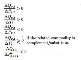
The Supply Function:
While analysing the relation between the quantity offered for sale and any of the determinants, economists usually focus upon the relation between quantity supplied and the product price. As the price of a product increases (decreases), more (less) is supplied by sellers, holding all variable constant.
The following definition is used in traditional economics:
Definition:
Supply is a list of prices and the corresponding quantities that a group of suppliers (firms) would be willing and able to offer for sale at each price at a particular point of time.
The supply functions may be expressed as:
ADVERTISEMENTS:
Qx= g(Px)
or supply can be specified by a schedule or a graph. Let us consider the market supply schedule for a good shown in Table 6.3. This table shows the minimum price necessary to induce firms to supply, per unit of time, for each of the six quantities listed.
In order to induce the firms to supply larger quantities, price has to rise. For example, if price increases from Rs. 4 to Rs. 5, firms will increase quantity supplied from 6,000 units to 6,500 units.

This schedule shows the minimum price acceptable to firms to supply each quantity shown in the list. Here we see that price and quantity supplied are directly related; as price falls firms supply less. To account for this we have to discuss the forces lying behind the law of supply, viz., cost of production.
At present we just assume that the supply schedule shows the minimum price necessary to induce producers voluntarily to offer each possible quantity for sale and that an increase in price is required to induce an increase in quantity supplied, other things remaining the same.
 If we plot all price-quantity combinations and join these points by a line we get a curve, viz., the supply curve. Thus the supply curve is a graphical representation of the supply schedule — a locus of points showing alternative price-quantity combinations. Since quantity supplied and price vary directly, the resulting supply curve slopes upwards from left to right.
Quantity Supplied and Supply:
Supply is a broad term referring to the entire supply curve of a commodity. On the other hand, the term ‘quantity supplied’ is interpreted narrowly. It refers to a particular point on the supply curve.
Recall that while deriving a supply schedule or drawing a supply curve we made the assumption that the other variables that affect the quantity offered for sale (technology, the prices of inputs, the prices of goods related in production, and price expectations) are held constant.
When the price of the commodity under consideration rises and firms are induced to offer a larger quantity for sale, we say that the quantity supplied increases. Conversely, if the price of the product falls, the quantity supplied decreases. Such an effect is illustrated in Figure 6.4. The original supply curve is S0S0‘. Now if the price falls from p to p’, the quantity supplied of x decreases along that supply curve from X0 to X’0.
If however, there is a change in any other variable (any other determinants of supply) firms are induced to offer more or less of the commodity at each price. In this case, we say that the original supply curve has shifted to a new position.
A decrease and increase in supply are illustrated in Figure 6.4 as a shift from S0S’0 to S1S’1 and S2S’2, respectively. (At the original price p, X1 units are supplied when supply decreases to S1S’1 and X2 units are supplied when the supply curve shifts to S2S’2).
An increase in supply may mean two things:
ADVERTISEMENTS:
(a) A larger quantity at the same price, or
(b) The same quantity at a lower price.
 The difference between movements along a given supply curve and changes (i.e., shifts) in the supply curve is not different from that in the case of the demand curve (schedule). Suppose that all factors that influence supply of a particular good are fixed and the price of the good falls. This is a case of movement down along the supply curve.
There is less quantity supplied at the lower price, but there is no change in the supply curve. There is no fall in supply because ‘supply’ is a broad term which refers to the entire schedule or to the entire supply curve. There is only a decrease in the quantity supplied.
When a determinant other than the price of the goods changes, there would be a change in supply, which refers to a change in the entire schedule or a shift in the entire supply curve to a new position. For example, suppose that the prices of paddy and jute double. Then, at any given price of wheat, suppliers would want to supply less wheat than before. In this case, the entire supply curve of wheat shifts to the left.
In Table 6.5, the effects of selected changes on the market supply of a hypothetical commodity, say X, are listed. The basic point is that the supply schedule or curve for good X is not changed or shifted by a change in its own price. The supply curve for good X is changed or shifted in response to changes other than a change in its own price.

Market Equilibrium:
When the supply and demand curves intersect, the market is said to be in equilibrium. This determines market price and quantity sold. Consider a hypothetical example. Suppose that in a market for some commodity, the demanders and suppliers have the particular schedules we previously set forth in Tables 6.1 and 6.3. These schedules are combined in Table 6.6.
We see that at only one price, Rs. 3, the equilibrium price, the market is cleared (quantity demanded equals supplied). At this price, the desires of buyers and sellers are simultaneously satisfied. It was Alfred Marshall who first demonstrated how the market forces driv7 the price towards the equilibrium level.
 Let us start with an arbitrary price say, Rs. 5. With this price, 3,000 units are demanded but 6,500 are offered for sale, leading to an excess supply (sometimes called a surplus) of 3,500 units. When there is excess supply, firms cannot sell all they wish at that price and they must cut price to clear their stock. Indeed, at any price above Rs. 3, there will be an excess supply (i.e., surplus) and price will fall to clear the market.
Alternatively, consider, the price Re. 1. Consumers are desirous of purchasing 6000 units, but producers are willing to offer only 3,000 units for sale creating an excess demand (a shortage) of 3,000 units.
Since their demands are not satisfied, consumers bid the price up. As they continue to bid up the price, quantity demanded decreases and quantity supplied increases until a price of Rs. 3 is reached and 5,000 units are sold per unit of time.
In Figure 6.5, DD’ and SS’, the market demand and supply curves, meet at a point E, the equilibrium point. Thus, Pe and Xe are the market-clearing (equilibrium) price and quantity, respectively. Only at a price of Pe does quantity demanded equal quantity supplied.

Suppose that price happens to be P1, which is greater than Pe. At P1, producers supply Xs but only Xd is demanded. An excess supply of Xd Xs exists. Thus, producers are forced to lower price in order to sell the entire amount they are willing to offer. At any price above Pe, there is an excess supply and producers will lower price.
On the contrary, suppose that price is P2. Demanders are willing and able to purchase X’d, while suppliers are only willing to offer X’s units for sale. There develops an excess demand of X’sX’d in the market. The unsatisfied buyers bid the price up. Any price below Pe creates an excess demand (i.e., shortage), and the shortage induces consumers to pay much to acquire the limited quantity that is available.
Given no external influences that prevent price from being bid up or down, an equilibrium price- quantity combination is attained. The equilibrium price is one that clears the market and there is neither excess demand nor excess supply in equilibrium
Thus, prices perform two functions. First, they act as a rationing device for the users of the product. If prices rise, they serve to determine who gets the products and, therefore, perform the service of ensuring that society allocates the product to its highest valued uses.
Secondly, they provide the inducement for sellers to supply more or less of the product according to the demands of the consumers. Prices rise, because consumers demand more of the good, and producers are induced to supply more. Falling prices give the signal that consumers demand less, and producers are induced to supply less of the good.

Given the above data concerning the demand for and supply of X in a given market:
(a) What would be the free market price of X?
(b) What would be the price if demand increased by 4 tons at every price?
(c) What would be the effect of a government’s imposing a minimum price of Rs. 5 per ton in the original situation?
Explain your answers.
Solution:
(a) Free market price is where demand equals supply, i.e., Rs. 3.
(b) If demand increased by 4 tons at every price market price would be where new demand equals supply, i.e., Rs. 4, since the demand and supply will now both be 14 tons.
(c) If the government imposed a minimum price, the equilibrium price of Rs. 4 per ton, this price would be above the free market equilibrium. If prices are held at this level suppliers are willing to produce more of the commodity than can be absorbed by the market. It will thus create a surplus of unsold stocks. This, situation can be dealt with by subsidizing exports of X so that the goods are sold at very low prices overseas.
Alternatively, the surplus of X can be destroyed or be given away in foreign aid programmes. A further possibility is for the government to establish production quotas for individual suppliers so that they each produce less than they would wish to produce at the government – fixed minimum price.
Comparative Statics:
So long we have examined a static situation for theoretical interest. However, in practice, managerial^ decision makers are frequently interested in the effect of changes in the determinants of demand and supply on price and on sales.
For example, we may raise such questions as: What will happen to the price of motor cars as the price of petroleum falls (or rises) or as income rises? What will happen to the quantity of furniture sold as the price of houses rises? What will happen to teachers’ salaries as there is spread of education in rural areas? All of these types of questions bear relevance for economic decision makers.
All such questions may simply be reduced to only one question of a general nature: What will be the effect on market price and output (sales) of changes in those determinants that cause a shift in the demand or supply curve? By comparing the market equilibrium positions before and after the changes, it will be possible to determine the direction, if not the magnitude, of such effects.
Recall that price adjustments occur along the prevailing demand and supply curves to eliminate shortages or surpluses. Thus, price and output are endogenous variables — variables determined from within the market system.
Certain variables which operate from outside the market system are exogenous variables (or environmental factors). In case of demand, such variables are the incomes of consumers, the prices of those commodities related in consumption to the good in question (i.e., substitutes and complements) taste, and consumer’s expectation about the future price of the commodity.
Likewise in the case of supply, the environmental factors are the level of available technology, the prices of inputs used In producing the commodity, the prices of those commodities that are related in production) to the one in question, and the producers’ expectations about the future price of the commodity. We have already examined how each of these variables will shift the demand curve or the supply curve.
We may now proceed a step ahead to examine the effects of shifts in the demand and/or supply curves. In Panel A of Figure 6.6, P0 and X0 are the equilibrium price and quantity when demand and supply are D0D’0 and SS’. Suppose demand decreases to D1D’1. At price P0, the quantity offered for sale exceeds the new quantity demanded by AB. That is, excess supply at P0 is AB.
Faced with this excess supply, producers reduce price until the new equilibrium is reached at P1 and X1. Alternatively, suppose that demand increases from D0D’0 to D2D’2. At price P0, quantity demanded exceeds quantity supplied, and a shortage occurs.
The shortage causes consumers to bid the price up until the new equilibrium at P2 and X2 is attained. It is clear that if supply remains fixed and demand decreases, quantity and price both fall; if demand increases, price and quantity both rise.
 Panel B of Figure 6.6 shows what happens to price and quantity when the demand curve remains unchanged but the supply curve shifts. Let the demand curve be DD’ and the supply curve S0S’0. The original equilibrium thus occurs at point E. Here price is P0 and quantity is X0. Now suppose the supply curve shifts to the left to S1S’1.
The shortage of CE at P0 causes consumers to bid up price until equilibrium is reached at the price P1 and quantity X1. On the contrary, if the supply curve shifts from S0S’0 to S2S’2 a surplus is created at P0 which causes producers to lower price.
Equilibrium occurs at F which corresponds to P2 and X2. Thus, we see that if demand remains constant and supply decreases, price rises and quantity falls; if supply increases, price falls and quantity increases.
Of course, both demand and supply can change simultaneously. In such cases the resulting changes in equilibrium price and quantity cannot be predicted accurately. The net effect largely depends on the relative strengths of the shifts in the two curves.
Complex Changes:
So long we were able to reach some firm conclusions in the analysis above because we stuck to the rule of ceteris paribus, i.e., of only considering one change at a time. But, in reality, more than one factor may vary.
Suppose, for example, that there is a large rise in the demand for apples because of a successful advertising campaign to promote them. This is followed by an unexpected bumper crop of apples. What will be the final effect upon the equilibrium price? See Fig. 6.7.

From Fig. 6.7 we will see that although the quantity demanded and supplied increases in both cases, in Fig. 6.7(a) the price falls while in Fig. 6.7(b) it rises. When multiple shifts in demand and supply curves are considered, we cannot reach any firm conclusion about the effect on the equilibrium price unless we know the precise magnitude of the changes.
This conclusion has consequences for any student appearing at an examination in economics. Suppose one is asked to consider the effect of a number of changes in the demand and supply of a particular product.
It is obvious from Fig. 6.7 that no firm conclusion can be reached unless both changes move in the same direction; for example, an increase in supply coupled with a decrease in demand will definitely lower the equilibrium price. What is the solution? The answer is to explain one change at a time.
In the example used above, for instance, first explain the effect of an increase in demand and draw a diagram to illustrate this. Then explain the effect of the increase in supply and draw another diagram to illustrate this. One has always to keep to the rule of explaining one thing at a time unless one has precise details of the demand and supply.
Price Ceilings and Price Floors:
In a market economy, prices serve two basic purposes:
(1) They ration scarce goods and services among consumers and
(2) They induce firms to produce more or less of a good or service.
Because of the Law of Scarcity, there is the need for a rationing system and an incentive system. Market prices act as devices for both.
However, sometimes the price system gives wrong signals and produces adverse outcomes. So it becomes necessary for the government to pass laws to fix minimum or maximum prices of commodities (like sugar) or factors (such as labour power).
But government price regulation is also likely to have certain undesirable effects on producers, consumers or labourers. And, in this context, Milton Friedman has rightly opined that “the neglect of indirect effects is the common sources of all fallacies.”
Government price fixation may be of two types — maximum legal price and minimum legal price.
Price Ceilings:
If the government fixes the maximum (ceiling) price below the equilibrium level, as in Fig. 6.8 there will be excess demand (shortage) of Qs — Qd. Black-marketing will develop, i.e., people will adopt some illegal means to pay more than the legal minimum price. In Fig. 6.8 some people will be eager to pay and end up paying a price (Pb) which is higher than the legal maximum price (Pc).
So the government has to allocate the commodity by introducing outright rationing. Thus price control is ineffective without rationing or administered allocation. In the absence of rationing we have the worst of both the worlds: a smaller quantity and a higher price.

Government price fixation may be of two types — maximum legal price and minimum legal price.
Other examples of such price controls are rent controls in large cities and ceiling on interest rates. To make interest ceiling effective the government may have to introduce a system of loan rationing.
Price Floors:
If, on the contrary, the government fixes a minimum prices by law there will be the problem of excess supply (surplus). But this problem arises only if the price is fixed above the equilibrium level, as Fig. 6.9 shows. Then there is an excess supply of Qs — Qd which has to be eliminated somehow.
The Government has to purchase the surplus from the market or restrict production of the commodity as is done in the USA in its agricultural programme (known as crop rationing).

An obvious example of such price floor is the system of support prices for various agricultural products. Another example is the minimum wage. If it is fixed above the equilibrium level there will be the problems of involuntary unemployment, as Fig. 6.10 shows.
Here we see that with the minimum wage (Wm) fixed above the equilibrium level (We), the number of persons employed will fall from Ee to Ed, but the number of unemployed persons will increase from zero to Es — Ed.
The portion of unemployment indicated by Es — Ed is due to an additional labour force participation which is induced solely by higher wages. Statistical studies corroborated this involuntary unemployment hypothesis.

Market Structures:
Business firms exist largely, if not entirely, to make profit. But the extent to which they succeed in fulfilling this objective depends on cost and demand conditions. Although cost conditions bear no relation to market structures, demand conditions depend largely on the market structure or the market conditions faced by the firm.
There are diverse market conditions in a market system. To be more specific, there are differences in the degree of competition found in various markets and industries throughout the economy. In essence, the structure of a market is the arrangement and interrelationship of firms in an industry.
In this text we shall look at four different abstractions, or models, and we will then refer to those different models as different market structures:
(1) Pure (perfect) competition,
(2) Monopoly,
(3) Monopolistic competition and
(4) Oligopoly.
Perfect Competition:
Perfect competition is the basis for the broadest and most important model of economic behaviour and market structure. It refers to “market conditions that provide an environment for a free, impersonal market in which the forces of demand and supply determine the allocation of resources and the distribution of income”.
This type of market is characterized by the existence of the following conditions:
(1) There is absence of government or any other form of control or intervention,
(2) A homogeneous product is traded. There is no product differentiation and no scope for advertising or sales promotion.
(3) There are innumerable buyers and sellers. Each one is so small a part of the market that it cannot alter the market price by selling or buying a little more or a little less. In other words, the market price is determined by the impersonal market forces. There is no collusion or control that influences the price.
(4) New firms are free to enter or old firms free to leave the industry and resources such as labour and capital are freely and perfectly mobile among employments and industries.
(5) Buyers, sellers and factory owners have perfect knowledge and information about prices, costs and wages. Most of these conditions are met in markets for agricultural commodities, the share market and the foreign exchange market. All other markets show various types of imperfections.
The outcome of a perfectly competitive market is a uniform market price for the homogeneous product. Any firm is at liberty to produce and sell all that it wants at the uniform price, but it can sell none of its product if its price is slightly higher.
Likewise any buyer can purchase any amount of a product at the uniform price, but none of the product at a slightly lower price. In essence, neither buyers nor sellers recognize any business rivalry or personal rivalry among themselves.
Monopoly:
Monopoly refers to a situation in which a single firm supplies the entire output of an industry. The monopolist is not bothered about the reaction of rivals because it has none. The presence of monopoly in a particular industry implies absence of a perfect substitute product. But to ensure this there must be some barrier to entry that keeps other firms out of the market.
However, it may be noted that while a monopolist has no direct competitors who sell the same product, a monopolist has indirect competitors. All other products are indirectly competitive with the product supplied by a monopolist in the sense that all goods and services compete for a limited amount of the consumer’s budget. Some products are no doubt closer substitute than others, but none is a perfect substitute.
Monopoly is a rarity. Public utilities such as the Calcutta Electric Supply Corporation (CESC) or Delhi Electric Supply Undertaking (DESU) are examples of monopolies. The DESU has been given the legal right to supply electricity to an entire market. However, their power over price and service is regulated and they face competition from supplies of substitutes such as natural gas and fuel oil.
Oligopoly:
Oligopoly refers to a market situation characterized by the existence of a few dominant firms of either homogeneous products (such as steel or aluminum) or differentiated products (like motor cars or cigarettes).
An important characteristic of oligopoly is mutual interdependence among the firms. An oligopolistic firm is a dominant firm in the sense that it is a large enough part of the market such that its decisions will effect the other firms in the industry.
Other firms do recognise this. Likewise, the other firms will react to decisions in a way that affects the oligopolistic firm, When Hindustan Motors Ltd. (HM) considers a price increase, an advertising campaign, development of a new model, a rebate or a financing plan, management has, of necessity, to consider reactions by Premier Automobiles Ltd. HM’s decisions will affect the demand for Premier Padmini and Maruti cars and PAL and Maruti Udyog’s reactions to HM’s decision will clearly affect the demand for Ambassador cars.
Monopolistic Competition:
Monopolistic competition refers to a market situation in which a large number of firms produce and sells somewhat similar but differentiated products. Each firm in this type of market is a monopolist in the sense that each one produces its own differentiated product. Only one firm produces Titan Watch, only one firm produces Colgate Toothpaste, only one firm produces Dettol, only one firm produces Cinthol soap.
Each of these firms is virtually enjoying a monopoly position on its brand- name product. But each firm has to face competition from rivals in the sense that firms compete with one another to sell products that are similar and clearly related. Each firm that produces cold drinks has a monopoly over production of its own product, but all firms that produce cold drinks compete to sell cold drinks.
There are more than a dozen producers of cold drinks in India. Yet, through advertising, Limca has succeeded in persuading consumers that its product is differentiated from other products, is somewhat more safe (because it is a zero bacteria drink).
Despite the fact the all cold drinks serve the same purpose, Limca has succeeded in capturing a large market share, and its producer is at the same time able to charge a relatively higher price. The following table gives a summary of the four major types of markets.
Case Study:
Vanaspati Decontrol:
In early 1986, the Government of India has removed the informal price control on vanaspati and reduced the quantum of imported oils being supplied to the vanaspati industry. With the revised policy, the vanaspati units will get 30 per cent of their requirement of raw materials from imported oils at Rs. 11,500 per ton.
Additionally, the industry has been allowed to lift up to 10 per cent imported oils at a commercial rate of Rs. 13,000 per ton in case of spurt in demand. This means, vanaspati units will have to obtain 70 per cent of their requirements from the domestic market.
The vanaspati industry has welcomed the new policy as it does away with the voluntary price control which had lost much of its relevance in recent times. The industry has also expressed the confidence that the new measure would create conditions for improvement in the quality of vanaspati and increase in its production.

During 1985, the Government had reduced in stages the share of imported oils supplied to the vanaspati industry. As late as January 1985, the industry was provided with 95 per cent of its requirements from imported edible oils at subsidised rates.
Gradually, the government reduced the imported oil component and also increased the issue price twice. In November last, the allocation of imported oils was reduced from 60 per cent to 50 per cent and the issue price was raised from Rs. 9,500 to Rs. 11,500 per ton. Besides, the term of voluntary price agreement had expired on January 1, 1986.
The Government’s policy of supplying imported edible oils to vanaspati units at subsidised rates has come under vehement criticism. It was claimed that the favoured treatment meted out to the industry in the matter of distribution of imported edible oils was neither justified on economic considerations nor warranted by the edible oil situation prevailing in the country.
As it is, vanaspati accounted for only 20 per cent of the edible oils and fats available in the country. Moreover, it catered to the needs of middle and higher income groups mostly in metropolitan and urban areas.
Thus, the benefit of government patronage through the supply of imported oils to vanaspati units has been mainly appropriated by the better off sections of consumers who could otherwise afford to pay higher prices for the cooking medium.
Despite the growing criticism, the Government continued to supply imported edible oils to the industry because, as the only organised sector in the vegetable oil industry, vanaspati provided a leverage for the government to check the open market prices of edible oils at least to some extent.
Whenever the open market prices rose much above a certain limit, the government started providing larger quantities of imported oils to the vanaspati industry, thus releasing local oils for direct consumption.
In 1985, when the supply of edible oils was comfortable and prices were ruling easy, the government reduced the supply of imported oils component to the industry with a view to propping up the prices of indigenous edible oils.
Moreover, the policy of voluntary price control which has been in force since 1979 had outlived its utility in recent years. Particularly, since 1983-84, oil supply has improved and the prices of edible oils have remained stable. During the greater part of 1985, the prices of vanaspati, a value added cooking medium, ruled below the prices of popular edible oils like ground-nut oil.
This has rendered the enforcement of voluntary price control on vanaspati irrelevant. Even in times of scarcity, the voluntary price agreement was more often than not flouted. This was because there was hardly any mechanism to control and monitor retail prices since the price agreement did not extend to the market place.
A reduction in the supply of imported oils to the vanaspati industry was necessitated by the deterioration in the foreign exchange resources of the country. During the first six months of the current financial year the trade deficit has amounted to Rs. 4,295 crores as against Rs. 2,807 crores during the same period a year earlier.
Given the foreign exchange constraints, the government is unlikely to resort to large imports of edible oils as in the past two years to bridge the gap in domestic production. It has in fact already made it every clear that imports of edible oils during 1985-86 will be cut and that the consumers will have to pay higher prices for edible oils which would in turn act as an incentive to the consumers.
As a sequel to this policy stance, the Government has decided to reduce the supply of imported edible oils to the vanaspati units. Besides, the decontrol of vanaspati is in tune with the recent policy of the government to remove controls on production and allow market forces to determine the prices.
Removal of voluntary price control does not imply that the government has abdicated its responsibility of ensuring the supply of vanaspati at reasonable prices to the consumers.
The government has in fact indicated that it will keep a close watch on the movement of vanaspati prices. The possibility of Government intervention in the event of either scarcity or unwarranted rise in the prices of vanaspati cannot altogether be ruled out.
In this sense the industry has been placed on trail and it might lose its freedom to adjust the scale of production and fix the prices of vanaspati if it tries to indulge in malpractices. In their own interest and to avoid the government interference, the vanaspati manufactures should evolve a code of conduct and try to operate within that framework.
A section of the trade has criticised the Government’s revised policy as it was announced at a time when the supply of edible oils is not expected to be very comfortable. The production of kharif groundnut has suffered a setback because of prolonged droughts in major producing states like Gujarat, Maharashtra and Karnataka.
However, the rabi outlook for oilseeds, particularly rapeseed and mustard seeds, is reported to be encouraging and hence a part of the shortfall in kharif production in 1985-86 would be about 126 lakh tons against the target of 133 lakh tons and the production of 130 lakh tons in 1984-85.
Moreover, in view of the foreign exchange constraints imports of edible oils are proposed to be slashed to 10 lakh tons against 13 lakh tons in 1984-85 and 16 lakh tons in 1983-84.
Despite the fall in the anticipated availability of edible oils, the vanaspati industry is not likely to face any serious shortage of its raw materials. Fortunately, the supply situation in respect of cottonseed oil, soyabean oil and rice bran oil used by the industry appears to be comfortable.
For the second year in succession, the country is posed to harvest a bumber crop of cotton. From this source alone about 2.5 to 3 lakh tons of oil will be available to the vanaspati industry.
The production of soya-bean oil which has been steadily increasing in recent years will meet part of the requirement of the industry. The industry produces about 9 lakh tons of vanaspati per annum.
Under the revised policy, it will get about 3 lakh tons of edible oils from imported sources and the industry is required to raise from other sources the balance of 6 lakh tons. Although the industry is not allowed to use groundnut oil and mustard oil, it can tap other sources of supply to meet a part of its requirements.
One of the criticisms levelled against the policy of supplying subsidised edible oils to the vanaspati industry and resorting to massive imports was that it has stunted the development of the oilseeds economy of the country. Continuing imports to meet the shortfall in domestic production had kept the prices of indigenous edible oils depressed which in turn acted as a disincentive to farmers to raise oilseeds production.
With the proposed cut in imports and the quantum of imported edible oils being supplied to the vanaspati industry, the prices of edible oils in the open market are likely to firm up. If the benefit of higher prices accrues to the farmers, it would act as a shot in the arms to the sagging oilseed economy in the country.
In its efforts to keep the vanaspati prices at competitive levels, the industry will be on the look-out for securing its raw material requirements from cheaper sources.
Pursuit of such an endeavour should boost the development of minor oilseeds of tree origin. Since a vulnerable section of society is engaged in collecting these oilseeds, the state governments can help the industry in tapping this rich but neglected source of oil.
If the potential of oil from seeds of tree origin is fully exploited, it will not only provide a supplementary source of raw material to the vanaspati industry but also reduce the country’s dependence on imports. In the context of the government’s decision to reduce imports and the anticipated shortfall in oilseeds production, the need to augment the production of oil from seeds to tree origin cannot be over-emphasised.
A section of the trade has expressed concern that the revised policy will boost the open market prices of edible oils and thereby fuel inflation. True, some increase in the prices of edible oils will be inevitable because of the tightening of supply.
But if the price increase persists and reaches alarming heights, the government may not hesitate to arrange more imports of edible oils to control runaway prices. However, modest increase in prices will ultimately put the oilseeds economy on a sound footing and help achieve a breakthrough in the production of oilseeds.
It is worth recognising that the impact of the policy of decontrol will not be even among different vanaspati units and among regions. The general feeling is that the benefit of the policy will be reaped mainly by big units to secure about 70 per cent of their edible oil requirements in the open market.
Similarly, the vanaspati units in the eastern region will have to procure bulk of their indigenous oil requirements from outside the region involving additional cost in manufacturing vanaspati.
According to one estimate, additional cost of transportation and sales taxes etc. would add up to Rs. 480 per ton of vanaspati. This will place the vanaspati units in the region at a disadvantageous position compared with the units in other states.
The Vanaspati Manufacturers’ Association has urged the Government to remove altogether the ceilings on the use of mustard and rapeseed oils by the vanaspati industry. The production of these oils had shown steady increase in recent years. Moreover the demand for these oils is regional and largely inflexible.
According to industry sources, the growers were not getting remunerative prices for these oils because of poor demand for direct consumption. The Association has, therefore, pleaded with the government to allow the vanaspati industry to use these oils as raw materials.
While welcoming the government’s decision to remove the informal price control and to reduce the quantum of imported oils, the Association has also pleaded for the abolition of excise duty on vanaspati industry. It may be recalled that the excise duty on vanaspati was raised from 5 percent ad valorem to 10 percent in the union budget for 1985- 86.
At the prevailing price, the excise duty amounts to Rs. 574 per ton or Rs. 24 per tin of 15 kg. Compared to this, refined oil bears a lower duty incidence of Rs. 106 per ton or Rs. 1.60 per tin of 15 kg.
The Association has also pleaded with the Government for the removal of curbs on the use of solvent extracted oils which will enable the solvent extraction industry to improve its capacity utilisation. Similarly, it has demanded the removal of restrictions on the production of vanaspati in pre-packaged consumer packs and production of groundnut refined oil, margarine and shortening.
At present, 30 per cent expeller mustard, rapeseed and toria oil and 10 per cent solvent extracted mustard oil is being allowed in the manufacture of vanaspati. The Government should consider raising this share of oil to enable the industry to meet its raw material requirements and produce vanaspati at a reasonable price.