Long Run Industry Supply Curve (With Diagram)

Let us learn about the Long Run Industry Supply Curve.

The long run supply curve of a competitive industry is not obtained in the same way as the short run industry supply curve. In other words, simply by aggregating individual firm’s long run MC curves one cannot obtain long run industry supply curve. The procedure of deriving the long run industry supply curve is different since, in the long run, entry into and exit of firms from the industry come into action.

A competitive firm in the long run produces at that point where the long run MC curve intersects the long run AC curve at the lowest point (i.e., P = AR = MR = LMC = minimum point of LAC). Thus, in the long run, a competitive firm operates its plant size optimally and efficiently.

In the long run, the supply of a commodity is determined by the minimum point of long run AC curve where optimum output is obtained. This results in a change not only in the size of the industry, but also in the supply of output. The change in scale of production in the long run brings about (external) economies and (external) diseconomies of production.

Long run industry equilibrium depends on such economies and diseconomies. That is why variation in cost occurs in a competitive industry in the long run. In other words, as industry output expands in the long run, a perfectly competitive industry may experience constant cost or decreasing or increasing cost.

How wills the long run AC curve of an individual firm shift as industry output expands depends on whether the industry operates under constant cost condition, or increasing cost condition, or decreasing cost condition. Consequently, the shapes of the long run industry supply curve will be horizontal, increasing, and decreasing—depending on the cost condition on which the industry operates.

A constant cost industry is one where cost structure of the individual firm remains stable as the industry expands its output. Prices of inputs employed by a constant cost industry do not change.

An increasing cost industry is one where cost of the individual firms rises as the industry expands its output. Here prices of inputs rise.

A decreasing cost industry is one where the expansion of output causes costs to decline. Under decreasing cost condition, prices of inputs decline.

Constant Cost Industry and the Horizontal Supply Curve:

A constant cost industry is one where expansion or contraction of the industry does not bring about a change in the prices of factors of production employed by it. Or, a constant cost industry may be defined as one where external economies and external diseconomies balance each other.

Expansion of a constant cost industry does create neither external economies nor external diseconomies. Consequently, cost stays at the same level as industry expands. Under constant cost industry, no matter how many firms leave or join the industry, every firm will retain the same set of cost curves (LAC and LMC) with which it started.

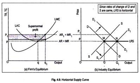
Fig. 4.6 demonstrates long run equili­brium of an industry operating under constant cost condition. Panel (a) of the figure shows long run equilibrium of a competitive firm while panel (b) describes industry equilibrium determined by the intersection of demand and supply curves.

Let us assume that DD and SS are the initial demand and supply curves. These two curves together determine (point TVF) equilibrium price at OP. Accepting this price, a typical firm would produce Oq output. Incidentally, all the firms are making zero economic profit since P = LMC = LAC.

If we assume that there are 10,000 identical firms in the industry, then the industry output would be Oq × 10,000 firms = OQ (shown in panel b). Since these firms are making only normal profit at the price OP, the industry is in equilibrium with an output OQ.

Now, let us suppose that there is an increase in market demand to D₁D₁ following an increase in money income or a change in the taste of buyers. As a result, market price rises from OP to OP₁ and the firm’s demand curve is now represented by P₁ = AR₁ = MR₁ line.

The firm will now expand its output to OQ₁. It will earn supernormal profit equal to the shaded area since P = LMC = MR₁ = AR₁> LAC. Existence of this profit implies that the industry is out of equilibrium. This will then act as an incentive for new firms to join the industry.

Two things will now happen. Firstly, demand for resources will go up. But, being a constant cost industry, input prices will remain unchanged. Thus, entry of firms will have no effect on cost curves. LAC and LMC curve will stay at the old level.

However, firms will continue to enter until excess profit disappears. Secondly, entry of new firms in the industry will shift the supply curve to S₁S₁. Industry equilibrium will now occur at point ‘N’ where the old price OP will be re-­established. At the price OP, OQ₁ output will be supplied in the industry.

If we connect the various market equilibrium points—’M’ and ‘N’—we get the long run industry supply curve (LRS) drawn in panel (b). Thus, under constant cost industry, the LRS curve is a horizontal straight line or perfectly elastic even though the short run supply has a positive slope.

Increasing Cost Industry and the Rising Supply Curve:

Sometimes, an expansion in industry output causes costs to rise in the long run. Thus as industry expands, external diseconomies outweigh external economies leading to a net increase in costs. As industry expands, demand for inputs rise and costs rise since the industry operates under increasing cost condition.

In other words, external disecono­mies cause LAC curve to shift upwards as industry expands. Consequently, the long run industry supply curve becomes positive sloping.

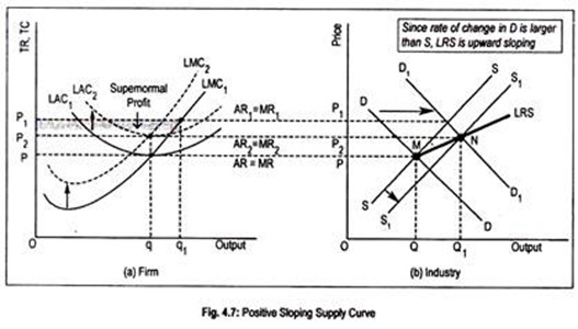
Fig. 4.7 illustrates the long run adjust­ment process of a competitive industry operating under increasing cost condition. Panel (a) shows long run equilibrium of a competitive firm and panel (b) shows industry equilibrium.

The industry is in equilibrium at the price OP and output OQ, as defined by the intersection of DD and SS curves at point ‘M’. Corresponding to this price OP, each firm produces Oq and is in long run equilibrium where P = AR = MR = LAC. Each firm is making only normal profit. Note that the industry output OQ = Oq × number of firms.

Suppose, demand curve now shifts to D₁D₁ following an increase in income of the buyers. The immediate impact of an increase in demand is the increase in price in the short run to OP j. This new price will be accepted by all the firms. This is represented by the demand curve P₁ = AR₁ = MR₁. Each firm will now produce OQ₁ and sell it at the price OP₁. Firms will now be making economic profit or pure profit (shaded area in the figure).

Now two things happen. Firstly excess profit will now attract new firms to join the industry. As new firms enter the industry there will be an upward pressure in the demand for inputs. This will cause input prices and, hence, costs, to go up. Their interconnected reaction will pull up the LAC and LMC curves to LAC₁ and LMC₁ in the leftward direction.

Secondly, the increased number of firms and increasing costs cause short run market supply curve to shift to S₁S₁. New supply curve S₁S₁ intersects the demand curve at point ‘N’. The industry equilibrium price and quantity are op₂ and OQ₁, respectively. At this price, no firms are making excess profit. The typical firm at the price OP₂ now produces Oq—the old level of output.

However, the output level that the firm now produces may be greater or less than the original one. Even then industry output is larger since more firms have joined the industry. Thus, industry output at the price OP₂ is Oq × number of firms = OQ₁. Now by joining points ‘M’ and ‘N’ we get a positive sloping LRS curve.

Alternative Explanation (Positive Sloping Supply Curve):

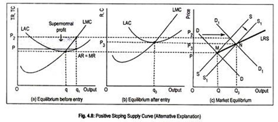
How is the upward rising industry supply curve derived under increasing cost condition has been alternatively demonstrated in Fig. 4.8. We know that, in the long run, firms enter the industry only when pure profit exists. Thus, pure profit is an incentive to join the industry. In Fig. 4.8(a) we have shown equilibrium of a firm before entry is made. Fig. 4.8(b) shows equilibrium of a newly entrant firm and Fig. 4.8(c) demonstrates long run industry equilibrium.

Let us assume that, initially, the competitive industry is in equilibrium at point ‘M’. The industry produces and sells OQ output at the price OP. As income increases, demand curve temporarily rises to D₁D₁ and short run equilibrium price rises to OP₂.

Each firm now produces and sells OQ₁ output at the price OP₂ (panel a). Firms are now making abnormal profit (shaded area in figure). This attracts new firms to join. In an increasing cost industry, as firms enter, demand for input rises, price of input rises, cost rises. This leads to an upward shift in the LMC and LAC curves as shown in panel (b). Costs will rise till excess profit vanishes.

At the new price OP₃, the firm earns normal profit after producing OQ₃ output. Further, entry of new firms in the industry leads to a rightward shift in the supply curve to S₁S₁. Finally, equilibrium is achieved at point W. The industry output is now OQ₃ and equilibrium price is OP₃. Now by joining these equilibrium points (‘M’ and ‘N’), we get an upward rising long run industry supply curve, labelled as LRS.

Decreasing Cost Industry and the Negative Sloping Supply Curve:

It may happen that when a new industry is established in a locality it may enjoy a situation of decreasing cost. A decreasing cost industry is one when expansion in an industry output causes input prices to fall, and, as a result, costs decline.

Or in a decreasing cost industry, external economies outweigh external diseconomies. As a result, both new and old firms of the industry find their LAC and LMC curves to shift in the downward direction, indicating a decline in cost.

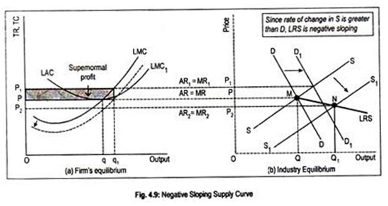
Fig. 4.9 explains this. As usual, panel (b) demonstrates industry equilibrium as defined by the intersection of the DD and SS curves. The industry is in equilibrium at point ‘M’. Corresponding to this equilibrium point, equilibrium output is OQ and equilibrium price is OP.

At this price, not only the competitive industry is in equilibrium but also all the firms within the industry are in equilibrium because P = AR = MR = LMC = LAC. The firm now produces and sells Oq output at the price OP and is enjoying only normal profit. Industry output is, thus, OQ = Oq × number of firms.

Suppose, demand curve shifts to D₁D₁ because of the increase in income of the buyers or increase in the price of substitute goods. The immediate reaction is the rise in price to OP₁. At this ruling market price, each firm produces and sells Oq₁ at the price OP₁ and enjoys some supernormal profit. This encourages firms to join the industry.

Two things will now happen. Firstly, because of the entry, demand for inputs will rise. But since the industry operates under diminishing cost, input price will decline and costs will decline. This is shown by the downward shift of the LAC and LMC curves to LAC₁ and LMC₁ (here the dotted curves).

Secondly, entry leads to an increase in the number of firms within the industry. This causes market supply curve to shift to S₁S₁. Final equilibrium is achieved at point ‘N’. Reduction in costs and increase in supply lead to a reduction in price to OP₂. At this price, the typical firm produces and sells Oq output and enjoys only normal profit.

There is now no incentive either to leave or join the industry. Though output of a firm stays at Oq, industry output is definitely larger because of the entry of new firms. Industry output as defined by the point ‘N’ of panel (b) is OQ = Oq × number of firms. By connecting these two equilibrium points— ‘M’ and ‘N’—we get a negative sloping industry supply curve, LRS.

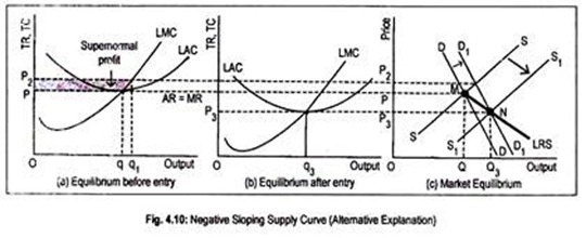
Alternative Explanation (Negative Sloping Supply Curve):

To derive a long run industry supply curve under decreasing cost, we use Fig. 4.10. Panel (a) shows equilibrium of a firm before entry, panel (b) explains equilibrium of a firm after entry takes place, and panel (c) describes overall industry equilibrium.

Let us assume first that the competitive industry is in equilibrium at point ‘M’. This means that the entire industry produces and sells OQ output at the price OP, panel (c). The corresponding equilibrium of a firm has been shown in panel (a) where it produces and sells Oq output at the price OP and earns only normal profit.

As demand curve now shifts to D₁D₁, the short run market price rises to OP₂. Each firm now produces and sells Oq₂ at the price OP₂ and gets abnormal profit. Abnormal profit (shaded area in figure) attracts more firms to join the industry. This causes input demand to rise first but input prices and, hence, costs, to fall since the industry is a decreasing cost one.

Newer firms now experience a lower cost compared to the old and existing firms. Further, entry causes supply curve to shift to S₁S₁. New supply curve S₁S₁ intersects D₁D₁curve at point ‘N’. Corresponding to this equilibrium point, equilibrium price is OP₃.

At this price, the firm produces and sells Oq₃ but manages only normal profit, leaving no further scope for either entry or exit. Industry output is now larger at the price OP₃. OQ₃ (= Oq₃ × number of firms) is the industry output. Now, by joining points ‘M’ and ‘N’, we get a supply curve which is negatively sloped, shown in panel (c).

Thus, an industry supply curve may be positive sloping in the short run but not in the long run. In the long run, the shape of an industry supply curve is governed by the cost condition in which an industry operates. It may be a horizontal one under constant cost industry, and negative sloping under decreasing cost industry.

It is to be remembered always that the long run industry supply curve cannot be derived from the LMC curve. The LAC curve determines the shape of the long run industry curve. Finally, positively sloped supply curve is the most relevant and a realistic one.