
Friedman-Phelps Model of Stagflation: Equations, Curves, Criticisms and Conclusion!
With the existence of stagflation, new economic models appeared during 1970s. M. Friedman and E.S. Phelps sought to explain the phenomenon of stagflation (or the instability of the Phillips curve) in terms of inflationary expectations; changes in inflationary expectations cause shifts in the Phillips curve.
According to the Friedman-Phelps model, the Phillips curve is wrongly specified because it is the real wage, and not money wage, that responds to the excess labour demand. The Phillips curve trade-off between money wage inflation and unemployment can exist only temporarily so long as the buyers and sellers of labour are fooled, i.e., so long as they both confuse money wages with real wages and do not correctly anticipate the inflation rate.
In other words, changes in money wage rates can offset the rate of unemployment only in the short run because it is only in the short run that employers and labourers confuse money wage changes with real wage changes and thus wrongly interpret inflation.
ADVERTISEMENTS:
For example, as a result of an expansionary monetary policy, an economy experiences price and wage inflation. This increase in money wages will be incorrectly interpreted by the producers as a reduction in the real wages and by the labourers as an increase in real wages.
The short run effect will therefore be an increase in both employment and the rate of inflation. It appears that the Phillips curve prediction is true i.e., inflation has led to a reduction in unemployment. But, this is only a temporary phase.
Eventually, the producers and the labourers will correctly learn about the higher rate of inflation. They will both incorporate this correct expectation into new labour contracts and the unemployment rate will return to its old natural level. Thus, there is no long run trade-off between inflation and unemployment.
The Friedman-Phelps model can be summarised in the following equation system:
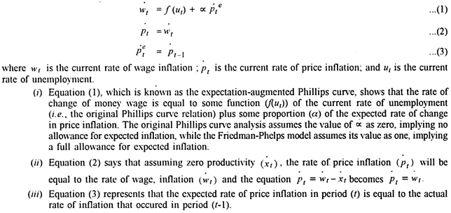
Thus, assuming that the rate of price inflation is equal to the rate of wage inflation, and that neither producers nor labourers suffer from money illusion, i.e., both correctly anticipate inflation, the Friedman- Phelps model implies- (a) that the anticipated changes in the price level will be fully incorporated into money wage contracts and (b) that, as a consequence, the rate of change of money wages will be a function of both the unemployment rate and the anticipated rate of prices.
Figure 10, which provides a graphic representation of Friedman-Phelps model, distinguishes between the short run and long run effects of unanticipated inflation. It is assumed that the natural, long run level of unemployment is un. ‘5 per cent’ Phillips curve shows the inverse short run relationship between actual inflation and unemployment when employers and employees anticipate an annual inflation rate at 5 per cent.
Along this curve, a temporary trade-off between inflation and unemployed exists because the actual rate of inflation differs from the anticipated rate and the employers and employees are fooled.
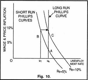
To start with, the economy is at point A, where the employers and employees correctly anticipate the 5 per cent rate of inflation and the unemployment rate is at its natural rate u„. Suppose that the unemployment rate is considered very high and an inflation rate of 10 per cent per annum is generated through a combination of monetary and fiscal measures.
If this new inflation rate is unanticipated by the employers and labourers, the economy will move from point A to point B and the unemployment will fall to u1. It appears that a 5 per cent point increase in inflation has been traded off for a decrease in unemployment rate from un to u1.
Eventually, both employers and labourers will realise that the actual inflation rate is 10 per cent per annum. New labour contracts will take this realisation into account and the unemployment rate will return to the natural level (5 per cent) and the economy moves from point B to point C.
Point C lies on ’10 per cent’ Phillips curve and at this point the actual rate of inflation (10 per cent) is correctly anticipated. Now, if unemployment is to be reduced, a still higher unanticipated rate of inflation is required.
Point A and point C are the points on the long run Phillips curve. Long run Phillips curve can be derived by finding the unemployment rate when the inflation rate is correctly anticipated. The long run Phillips curve is vertical and its position is determined by the natural rate of unemployment.
In this long run, there is no tradeoff between inflation and unemployment. Thus, the Friedman-Phelps model can explain the existence of (a) short run Phillips curve and (b) a long run Phillips curve based on a set of shifting, unstable Phillips curves.
The policy implication of the Friedman-Phelps model is that monetary policy (or fiscal policy) can affect employment and output in the short run because these policies can fool the people, i.e., can lead people to make errors in anticipating inflation, in the short run.
But, in the long run, these policies will become ineffective because, in the long run, employers and employees will fully and correctly anticipate the inflation rate and as a consequence, unemployment will return to its natural rate.
ADVERTISEMENTS:
Friedman-Phelps model is based on the notion of natural rate of unemployment. It is the rate of unemployment to which the economy returns in the long run after the stabilisation policies are correctly anticipated by the people.
The natural rate of unemployment consists of two kinds of unemployment:
(i) Frictional unemployment or the type of unemployment experienced by people who are between steady jobs.
(ii) Unemployment due to rigidities in the economic system and its interferences with labour mobility or wage rate changes.
ADVERTISEMENTS:
Various rigidities and interferences are:
(a) Union activity which restricts supply of labour;
(b) Licensing arrangements granted by regulatory agencies;
(c) Minimum wages laws and
ADVERTISEMENTS:
(d) Welfare system that reduces incentives to work.
According to Friedman, stabilising policy can affect only frictional unemployment and that also temporarily by fooling the buyers and sellers of labour. Phillips curve trade-off simply represents a temporary change in the frictional unemployment.
Friedman-Phelps model can be alternatively explained with the help of aggregate demand and aggregate supply curves of labour. In Figure-11 A, aggregate demand and aggregate supply curves of labour (D0 and S0 curves) of the classical model are given. N0 is the full employment level which also implies natural rate of employment.
Real wage rate is w0. In Figure-11 B, these curves have been multiplied by the initial price level (P0). Thus, at the initial equilibrium, employment is N0 and the nominal wage rate is W0. Now the aggregate demand is increased to D1, as a result of which the price level increases to P1.
D1P1 is the new demand curve. Increased demand for labour induced a rise in nominal wages from W0 to W1, and in employment from N0 to N1. At this stage, workers have not realised that prices have risen. They, therefore, increase labour supply by moving upward along S0P0 curve.
ADVERTISEMENTS:
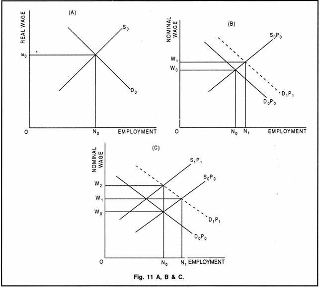
But, in the long run, the increase in prices will be fully reflected in the supply curve, which will shift leftward from S0P0 to S1P1 (as shown in Figure-11C). The effect of this shift will be to put more pressure on nominal wages, causing them to rise to W2. The employment comes back to its initial level N0.
Thus, the upward shift in the demand curve is completely offset by an equal upward shift in the supply curve. The end result of all this is that prices and nominal wages have risen, but the real wage and the level of employment remain unchanged.
Friedman-Phelps model of stagflation has been criticised on the following grounds:
1. Persistence of Unemployment:
ADVERTISEMENTS:
Friedman-Phelps model fails to provide proper explanation for the persistence of unemployment at levels either above or below the equilibrium or natural rate. According to this model, unemployment persistence is caused by delays in the flow of information generated endogenously in the model by the inflationary or deflationary surprises.
But, unfortunately, the delay is not generated endogenously by the model and its length is a matter of judgment. Thus, it is difficult to test how much of the observed variance in unemployment can be attributed to inflationary or deflationary surprises.
2. Degree of Adjustment to Inflation:
Friedman-Phelps model depends crucially on a specific assumption regarding the degree of adjustment of expected inflation to actual inflation (or the value of ∝ in the model).
There are three possibilities:
(i) α in the model can take the value unity, which implies that expected inflation is fully incorporated into current wage changes, so that there is absence of money illusion; there is no trade-off between inflation and unemployment in the long run and the Phillips curve is vertical.
ADVERTISEMENTS:
(ii) If, on the other extreme, α takes the value zero, then Phillips’ original formulation is correct which means that there is only one negatively sloping Phillips curve regardless of price expectations; inflation-unemployment trade-off exists and workers have money illusion.
(iii) In between these two extreme cases is the situation in which 0 < ∞ < 1, which means that there is partial but not complete compensation for anticipated inflation. This case implies that there is a long-run Phillips curve which, although more steeply sloped than the short-run ones, is not vertical; there is some trade-off between inflation and unemployment, and workers have money illusion even in the long-run.
Friedman-Phelps model, with its prediction that there is no inflation-unemployment trade-off in the long- run, is based on the assumption of α = 1 (i.e., first possibility) and ignores the other possibilities (i.e., second and third).
3. Empirical Evidence:
What is the actual value of α in the actual world is an empirical question. Majority of the research studies have shown that α falls in the range between .3 to .8, implying the existence of a negatively sloping long-run Phillips curve. Such findings suggest that, while people are rational and do adjust to inflation, they are subject to some degree of money illusion and do not therefore fully adjust to inflation.
4. Implication about Money Illusion:
ADVERTISEMENTS:
Even if the degree of adjustment to inflation (value of α) is significantly less than unity or nearly zero, this need not necessarily imply the presence of money illusion. In case where the wage is determined by collective bargaining, the workers may, for some reason, be prevented from fully incorporating their inflationary expectations into money wage settlements.
For example, Rees argued that the transactions costs involved in continuously adjusting the real wage under inflationary conditions may be sufficiently high to discourage complete adjustment for expected inflation.
5. Formation of Expectations Criticised:
Friedman-Phelps model assumes that expectations are generated according to the adaptive expectations mechanism which implies that current expectations are equal to the weighted average of past rates of inflation.
This assumption has been challenged by the recent development of the concept of rational expectations, according to which expectations are formed rationally on the basis of an economic model of the determination of the variable in question, rather than on the basis of weighted average of past values of the variable.
6. Rational Expectations Hypothesis:
Friedman-Phelps, model maintains that monetary policy can affect real variables like employment and output only in the short run, because people can be fooled only in the short run, and not in the long run. According to the rational expectations hypothesis, the stabilisation policies cannot systematically fool people.
For example, monetary policy cannot lead people to wrongly estimate the rate of inflation; some will underestimate and others will overestimate. This implies that the stabilisation policy cannot systematically influence employment and output even in the short run.
7. Vague Concept of Natural Rate of Unemployment:
The concept of natural rate of unemployment on which the Friedman-Phelps model is based has been criticised on the ground that it is a vague concept. It has not been defined in specific terms.
Tobin suggested a compromise between the negatively sloping and vertical Phillips curves. His modified Phillips curve is vertical at low levels of unemployment and becomes negatively sloping at relatively high levels of unemployment (as shown in Figure-12).
The vertical portion of the Phillips curve at U0 level of unemployment indicates that there exists no trade-off between inflation and unemployment. The negatively sloping portion of the Phillips curve beyond U0 level of unemployment indicates that there exists a trade-off between inflation and unemployment at higher levels of unemployment.
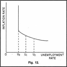
It means that at higher levels of unemployment increasing inflation will reduce unemployment (from U2 to U1 and to U0). This might be due to the downward stickily nature of wages; workers resist a decline in the wages. At U0 level of unemployment, the curve becomes vertical.
This implies that as unemployment falls to U0, the tradeoff between inflation and unemployment disappears, implying that changes in the rate of inflation no longer affect the level of unemployment. At very low levels of unemployment, further employment may not be provided because of imperfections of labour market.
Broad conclusions of the Friedman-Phelps model of stagflation are given below:
(i) The phenomenon of stagflation (or the instability of the Phillips curve) has been explained in terms of inflationary expectations. In other words, change in inflationary expectations cause shifts in the Phillips.
(ii) The problem of stagflation cannot be solved by adopting a stabilisation policy.
(iii) Demand-management (monetary and fiscal) policies should be aimed at achieving stable and lower inflation, and not at reducing unemployment rate.
(iv) Supply-side policies, such as changes in the tax structure to improve incentives to work and return to investment, may be more successful in increasing employment.