Tobin’s Portfolio Balance Approach (With Diagram) | Demand for Money

Let us make an in-depth study of the Tobin’s Portfolio Balance Approach.

The main problem with Keynesian approach to the demand for money is that it suggests that individuals should, at any given time, hold all their liquid assets either in money or in bonds, but not some of each.

This is obviously not true in reality.

The second approach — Tobin’s model of liquidity preference — deals with this problem by showing that if the return on bonds is uncertain, that is, bonds are risky, then the investor worrying about both risk and return is likely to do best by holding both bonds and money.

Portfolio theories like the one presented by Tobin emphasises the role of money as a store of value. According to these theories, people hold money as part of their portfolio of assets. The reason for this is that money offers a different combination of risk and return than other assets which are less liquid than money — such as bonds.

To be more specific, money offers a safe (nominal) return, whereas the prices of stocks and bonds may rise or fall. Thus Tobin has suggested that households choose to hold money as part of their optimal portfolio.

Portfolio theories predict that the demand for money depends on the risk and return associated with money holding as also on various other assets households can hold instead
of money. Furthermore, the demand for money should depend on real wealth, because wealth measures the size of the portfolio to be allocated among money and the alternative assets.

For instance, the money demand function may be expressed as:

(M/P)_d = f(r_s, r_b, π^e, W)

where r_s = the expected real return on stock, r_b = the expected real return on bonds, π^e = the expected inflation rate and W= real wealth. An increase in r_s or r_b reduces money demand, because other assets become more attractive. An increase in n^e also reduces money demand, because money becomes less attractive. An increase in W raises money demand, because higher wealth means a larger portfolio.

It is against this backdrop that we study the portfolio theory of money demand.

Speculative Demand for Money as Behaviour toward Risk:

Tobin ignored the determination of the transactions demand for money and considered only the demand for money as a store of wealth. The focus is on an individual’s portfolio allocation between money-holding and bondholding, subject to the wealth constraint, i.e., W = M + B, where W is the total fixed wealth, M is money and B is bond.

In Tobin’s theory there is no such thing as fixed normal level to which interest rates are always expected to return as has been postulated by Keynes. Following Tobin we can assume that the expected capital gain is zero. This is because the individual investor expects capital gains and losses to be equally likely.

The best expectation of the return on bonds is simply the prevailing market rate of interest (r). But this is just the expected return on bonds. The actual return also includes some capital gain or loss, since the interest rate does not generally remain fixed.

Thus bonds pay an expected return of interest, but they are a risky asset. Their actual return is uncertain due to the fact that the market rate of interest fluctuates even in the short run.

In contrast, money is a safe asset because it yields no return at all. At the same time money is a safe asset since no capital gain or loss is made by holding money. In Tobin’s view an individual will hold some propor­tion of wealth in money for reducing the overall riskiness of his portfolio.

If only bonds are held, returns would be maximum no doubt but the risk to which the investor is exposed will also be maximum. A risk- averse investor would voluntarily sacrifice some return for a reduction in risk. Tobin argues that money as an asset is demanded as an aversion to risk.

Tobin’s theory is explained in Fig. 19.4. On the vertical axis of the upper quadrant we measure the expected return to the portfolio; on the horizontal axis we measure the riski­ness of the portfolio. The expected return on the portfolio is the interest that can be earned on bonds.

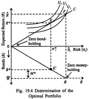
This depends on two things: (i) the interest rate and (ii) the proportion of the portfolio held in bonds. The total risk to which an individual is exposed depends on (i) the uncertainty concerning bond prices — that is, the uncertainty concerning future movements in market rate of interest, and (ii) the proportion of the portfolio held in bonds.

Let us denote the expected total return by R and the total risk of the portfolio as a σ_t. If an individual holds all his wealth (W) in money and none in bonds, i.e., W = M + 0, both R and σ_t will be zero, as shown by the origin (point 0) in Fig. 19.4. With an increase in the proportion of bonds, i.e., W = M + B; as M falls and B increases, R and a, will both rise.

The opportunity line C is a locus of points showing the terms on which the individual investor can increase R at the cost of increasing σ_t. A movement along C from left to right shows that the investor increases his bond holding only by reducing his money holding.

The lower quadrant of Fig. 19.4 shows alternative portfolio allocations, resulting in different combinations of R and σ_t. The vertical axis measures bond holding. The amount of bonds (B) held in W increases as the investor moves down the vertical axis to a maximum of W.

The difference between W and B is the asset demand for money (M). The line OB in the lower part of the diagram shows the relationship between a, and B. As the proportion of B in W increases, σ_t also increases. This means that as the proportion of bonds in the portfolio increases, the total risk of the portfolio increases, too.

Preference of the Investor: Risk-Aversion:

The optimal portfolio allocation depends on the preferences of the investor. Here we assume that the investor is risk-averse. He wants the best of both the worlds — a high return on the portfolio by avoiding risk. He will accept more risk if he is compensated by an increase in expected return. Let us assume that the utility function of the investor is U = f(R, σ_t) …(9)

where an increase in R increases utility (U) and an increase in σ_T reduces U. In Fig. 19.4 we show three indifference curves of the investor for three levels of utility U₁, U₂ and U₃. Each indifference curve shows the risk-return trade-off, i.e., the terms on which the investor is desirous of taking more risk if compensated by a higher expected return.

All the points on any such indifference curve yield the same fixed level of utility.

Any movement from U₁ to U₂ and from U₂ to U₃ implies higher level of utility, i.e., higher levels of R and the same or even lower levels of σ_t. The indifference curves are upward sloping because the investor is risk-averse. He will take more risk only if compensated by a higher return. Moreover, the curves become steeper as the investor moves to the right, implying increasing risk aversion.

If we make this assumption, then the more risk the individual has already taken on, the greater will be the increase in expected return required for the investor to be exposed to a
greater degree of risk. We may now determine the optimal portfolio allocation of a risk averse investor.

Optimal Portfolio Allocation:

A risk-averse investor will move to that point along the line C which enables him to reach the highest attainable indifference curve. At that point he ends up choosing that portfolio which he intends to choose and, thus, maximises his utility. The reason is obvious. At the

tangency point E, with R = R* and σ_t = σ*_t, the terms on which the investor is able to increase expected return on the portfolio by taking more risk, shown by the slope of the line C, is equated to the terms on which he (she) is willing to make the trade-off, as is measured by the slope of the indifference curve.

From the lower part we see that this risk-return combination is achieved by holding an amount of bonds equal to B*, and by holding the remainder of wealth (W̅ – B* = M*) in the form of money.

The demand for money thus shows the investor’s ‘behaviour towards risk’, i.e., the result of seeking to reduce risk below what it would be if W̅ = B and M = 0. In Fig. 19.4 such an all-bonds-portfolio would be associated with risk of σ_t and the expected return of R, as shown by point F in the upper part of the diagram.

This portfolio yields a lower level of utility than that represented by bond holdings of B* and money holdings of M*.

The reason is that as the investor moves to the right of point E along the line 0C, the additional return expected from the portfolio by holding more bonds (and less money) is not adequate to compensate the investor for the additional risk (the slope of the line 0C is less than that of the indifference curve U₂). The movement to point F takes the investor to a lower indifference curve, U₁.

Interest Rate Changes and the Speculative Demand for Money:

In Tobin’s theory the amount of money held as an asset depends on the level of the interest rate. Fig. 19.5 shows the relationship between interest rate and asset demand for money. An increase in the rate of interest from r₀ to r₁ and then to r₂ will improve the terms on which the expected return on the portfolio can be increased by taking more risk.

So the line 0C becomes steeper. It rotates anti­clockwise from C(r₀) to C(r₁) and then to C(r₂).

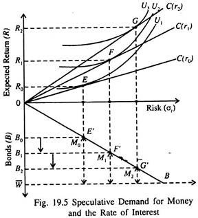
The investor responds by taking more risk and earning higher expected returns by moving from E to F and then to G. It may be noted that each point is one of portfolio optimisation. In this case his holdings of bonds (risky asset) increase (from B₀ to B₁, and then to B₂) and money holdings fall (from M₀ to M₁, then M₂).

In short, as the interest rate rises, a given increase in risk, which corresponds to a given increase in the amount of bonds in the portfolio, will result in a greater increase in expected return on the portfolio.

Comments:

In Tobin’s theory, like that of Keynes, the speculative demand for money varies inversely with the interest rate. The reason is that an increase in the rate of interest implies an increase in the payment received for taking more risk. When the interest rate increases, the investor is eager to put a larger proportion of his portfolio into the risky asset, bonds — and thus a smaller proportion into the safe asset — money.

From the portfolio theories, we can look at the money demand function (M/P)_d = f(Y, i) as a useful simplification. First, it uses real income Y as a proxy for wealth’ W. Secondly, the only return variable it includes is the nominal interest rate, which is the sum of the real return on bonds and expected inflation (that is, i = r_b+ π^e). The portfolio theories suggest that the demand function for money should also include the expected returns on other assets as well.

Are portfolio theories really useful for studying the demand for money? It depends on which measure of money we are considering. If we consider any narrow money (M₁), it is to be treated as a dominated asset, in the sense that as a store of value, it exists along with other assets that are always better. Thus, as Mankiw has suggested: “It is not optimal for people to hold money as part of their portfolio, and portfolio theories cannot explain the demand for these dominated forms of money.”

It may also be added that portfolio theories are more plausible as theories of money demand if we adopt a broad definition of money. Although the portfolio approach to money demand may not be plausible when applied to M₁, it can suggest a clear explanation of the demand for M₂ or M₃.

Tax Rates and Portfolio Choice:

A major portion of the revenues to a successful investment goes to the government as taxes. Since different assets are treated differently by the tax laws, tax considerations are obviously important in choosing a portfolio. After all, rational investors care about after-tax returns, not before-tax returns.

Government bonds illustrate this point. These bonds yield a lower return than do corporate bonds (debentures) of comparable risks and liquidity. Still, people buy government bonds because they are generally exempt from income tax and capital gains tax. The higher an investor’s income, the more valuable these tax exemptions are, because his tax savings are greater the higher the tax rate.

The higher demand for these tax-exempt bonds from high income investors pushes up their price, which reduces the return received on the bonds. We can expect the return to decline to the point where the after-tax return for high income individuals is at most slightly higher than for an ordinary taxable bond of comparable risk.

Loss Offset and the Return to Risk:

No financial investment gives a guaranteed rate of return and an individual who buys equity shares undertakes a risk. No investment is a safe bet. In other words, to make an investment is to gamble, and the investors should be interested in the gamble only if the value of probable gain outweighs that of probable losses.

Since an investor’s marginal utility of money income falls, an even-money or a fair bet (in which there is fifty-fifty chance of winning or losing) may not always be acceptable. If a tax on investment income worsens the odds by reducing the expected return, investment will fall. But such a tax may not always reduce the odds. It will reduce the investor’s return if he wins.

However if a loss offset is allowed for, it will also reduce his loss if he loses. Given a proportional tax, both are equiprobable events. Both probable gains and probable losses will be reduced at the same rate. The tax may induce an investor either to increase or to reduce his risk-taking — depending on circumstances.

The possibility of increased risk taking is shown in Fig. 19.6 where the rate of return is measured on the vertical axis and the risk is shown on the horizontal axis. Let us suppose, for the sake of simplicity, that the investor chooses between holding cash (which is completely safe) and a single alternative, say a cor­porate bond, of given risk.

The opportu­nity line 0A shows the combinations of risk and return available to him by choos­ing different mixes of cash and bonds. With 100% cash holding, he will stay at point zero where he assumes no risks and receives no return either. If all his funds are invested in bonds he will move to point B, with risk 0C and return 0D.

Before tax the investor is at point E₁ at which his opportunity line 0A just touches the highest attainable indifference curve U₂. His risk equals 0F and return is 0G. Here the indifference curve is drawn so as to show the increasing risk aversion.

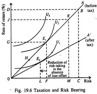
Successive increases in risk call for rising additions to the rate of return if the investor is to remain equally well-off. This follows from the implicit assumption that the utility of income schedule rises at a decreasing rate as income increases.

Now a 50% tax is imposed and we assume that full loss offset is allowed. If the investor does not change his portfolio mix, he will now find himself with half the risk and half the return than he had before, i.e., in a position similar to that provided by portfolio mix H prior to tax.

Since before the imposition of the tax he could have improved his position by moving from point H to tangency point he will now prefer to move from E₁ to K. At K gross risk and return have doubled but his net risk and return are the same (i.e., what they were at U₂ — before the imposition of the tax). No doubt his private risk taking has remained unchanged. But total risk taking, as seen from the point of view of the economy as a whole has increased. The reason is that the government has now become a partner. It now takes half the return and assumes half the risk, too. This outcome is conceivable only if loss offset is permitted.

Without loss offset, the tax would rotate the opportunity line from 0A to 0A’ and the new equilibrium would be at a tangency point E₂, with risk taking decreased to 0L.

Under certain conditions, a tax with loss offset will increase risk taking. The investment choice is not just one between cash (assumed to be riskless) and one risky asset. Inflation renders cash holdings risky, and choices among alternative risky assets are to be considered.

The outcome then depends on the precise nature of the investor’s preferences or the shape of his indifference curves. The net result may be either to increase or to reduce risk taking — and no simple generalisation regarding the outcome is possible.