Determination of Demand for Money and Behaviour of Velocity | Demand for Money

Let us make an in-depth study of the Determination of Demand for Money and Behaviour of Velocity.

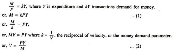
We know that the demand for real money balances (M_d/P) must equal the supply (M/P). Therefore,

For simplicity, if we assume that P is constant, then real spending will remain constant over the year, too.

(a) From equation (1) or (2) we find the link between the demand for money and the velocity of money. When people want to hold a large amount of money for each rupee of income (k is large) money changes hands less frequently (V is small). The converse is also true.

When people want to hold only a little money (k is small) money changes hands frequently (V is large).

In other words, an increase in k (which is an indicator of increased transactions demand for money) implies a decrease in velocity of money (V). So the strength of liquidity preference (which indicates the fraction or proportion of money people hold in the form of liquid balance) and the velocity of money V are the two sides of the same coin (since Vis the reciprocal of k).

We can use the formula for the optimal number of trips to express velocity as a function of expenditure, the interest rate and the cost of trips to the bank. The formula for the optimal number to trips N is

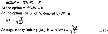
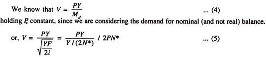
So we have expressed velocity as a function of the number of trips to the bank. Here V = 2PN*, i.e., doubling the number of trips to the bank will double V. This result follows from the fact that for any N, the average amount of money held is Y/(2N). If N increases, Y/(2N) will fall. This is equivalent to a rise in V because, when people hold a small amount of money for every rupee of income or expenditure Y, k will be small but V will be large — since k = 1/V.

i. Interpretation of the Result:

Now V is a function of Y, F, and i. Equation (3) suggests that an individual holds money if expenditure Y is higher, if the interest rate i is lower or if the fixed cost of going to the bank F is higher.

(i) If the interest rate rises the transactions demand for money will fall. Therefore, the velocity of money will rise.

(ii) If the price level rises, people require more money for transaction purposes to be able to buy the same quantity of goods and services. As a result k increases and V falls.

(iii) If the number of trips to the bank (N) is fixed rather than discretionary, then N responds only to changes in expenditure (Y), but not to the interest rate (i). This means that average money holdings (Y/2N) are proportional to expenditures and are insensitive to the interest rate.

Thus, if Y increases, (Y/2N) will increase proportionately and are velocity will fall correspondingly. But a change in i will have no effect on N and, thus, on (Y/2N). Thus interest rate changes will have no effect on velocity. In other words, the velocity will remain constraint.

ii. Theory and Evidence on Transactions Demand for Money:

The transactions demand for money responds to changes in income and the rate of interest. The income elasticity of transactions demand for money as also the interest elasticity of such demand determine the slope of the LM curve and, thus, determine the relative effectiveness of monetary policy and fiscal policy.

The Baumol-Tobin model’s square-root formula simply suggests that the income elasticity of money demand is ½: a 10% increase in income will lead to only 5% increase in demand for real balances. It also suggests that the interest elasticity of money demand is ½: a 10% increase in interest rate will lead to just 5% fall in (M_d/P).

Most statistical studies of demand for money do not support these predictions. In reality the income elasticity of money demand is found to be larger than ½, while interest elasticity is found to be smaller than ½. So the model is not fully correct.

One reason for the failure of the model is that some people enjoy much discretion over their money holdings, as has been hypothesised by the model. For instance, we may think of a person who has to go to the bank once a month to deposit his salary cheque.

While at the bank he withdraws just enough money needed for the next 30 days (until he receives another cheque on the next pay day). For this person, the number of trips to the bank, N, remains fixed — irrespective of his expenditure (10 or the interest rate (i). This means that his average money holdings (Y/2N) are exactly proportional to Y and completely unresponsive to i.

A Weighted Average of Money Demand:

Now let us consider a small community where two different types of people live. The first group is assumed to have income and interest elasticities of transactions demand for money of ½ as has been predicted by the model. The other group has a fixed N. So for them income elasticity of demand for money is 1 but interest elasticity is zero.

This means that the overall demand for money will be a weighted average of the demands of both the groups. The income elasticity will lie in-between ½ and 1 and the interest elasticity will be between j and zero. Empirical studies have found these values.